Flow parsing as causal source separation allows fast and parallel object and self-motion estimation

Abstract

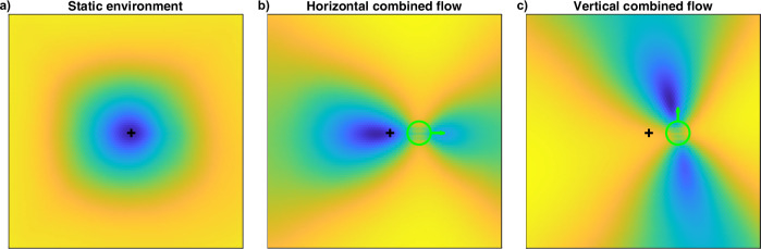
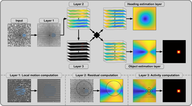
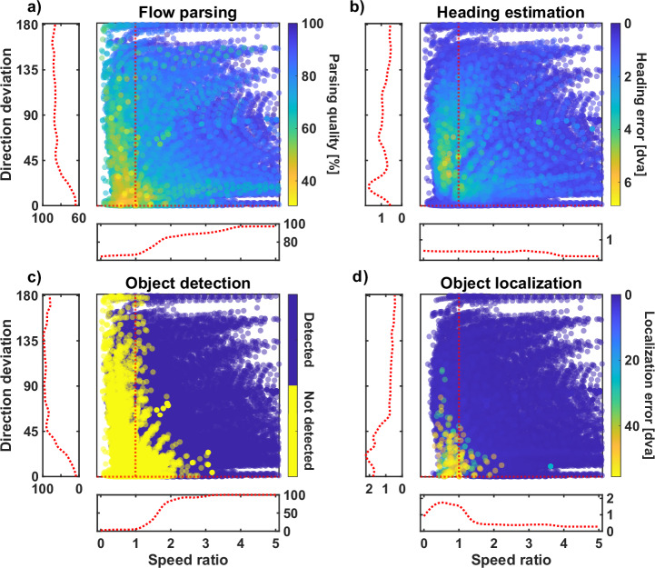
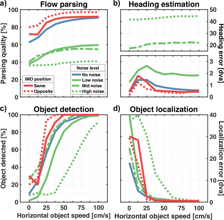
Optic flow, the retinal pattern of motion experienced during self-motion, contains information about one's direction of heading. The global pattern due to self-motion is locally confounded when moving objects are present, and the flow is the sum of components due to the different causal sources. Nonetheless, humans can accurately retrieve information from such flow, including the direction of heading and the scene-relative motion of an object. Flow parsing is a process speculated to allow the brain's sensitivity to optic flow to separate the causal sources of retinal motion in information due to self-motion and information due to object motion. In a computational model that retrieves object and self-motion information from optic flow, we implemented flow parsing based on heading likelihood maps, whose distributions indicate the consistency of parts of the flow with self-motion. This allows for concurrent estimation of heading, detecting and localizing a moving object, and estimating its scene-relative motion. We developed a paradigm that allows the model to perform all these estimations while systematically varying the object's contribution to the flow field. Simulations of that paradigm show that the model replicates many aspects of human performance, including the dependence of heading estimation on object speed and direction.

Fig. 1. Examples of residual surfaces.

Corresponding flow fields are due to simulated observer translation towards a static cloud of dots. The black plus indicates the FOE of the radial flow pattern and, therefore, the heading direction. The object, if present in the scene, is depicted with a green circle, and the green arrow indicates the direction of the combined flow. a The residual surface has a singular peak, which coincides with the true heading direction when no object is present. b, c When present, a moving object gives rise to residual surfaces with a saddle point at the object’s location, and the position of the surrounding peaks changes with the object’s flow direction.

Fig. 2. Structure of the computational model.

The model processes optic flow to detect the presence of a moving object, estimate self-motion direction, estimate object motion direction, and determine object location. It consists of multiple layers with specific processing operators in each layer. Optic flow fields form the input into the model. White and blue vectors represent observer flow and combined flow, respectively. Layer 1 computes a vector representation of the input flow by computing local averages of speed and direction. It contains operator units with small circular receptive fields that cover the FOV. The black circle shows the receptive field of one operator as an example, and the locations of the remaining operators are indicated with black dots. Layer 2 computes residual surfaces for flow in different parts of the visual field. Flow vectors in the receptive field of one operator are grouped, and one residual surface is computed for each group. Layer 3 computes activity maps, one for each residual surface. Operators calculate average residual values in parts of their cross-shaped receptive fields and use differences between them to compute activity. Receptive fields vary in size and orientation and cover the residual surface. The flow parsing process is based on the activity maps and decides whether a residual surface is used for heading or object estimation. The corresponding surface is used for object estimation when the activity maximum is high enough. The heading estimate is determined by the peak of the heading map, which is the result of summing the respective surfaces. For the object estimation, the incoming surfaces are summed up, and an activity map is computed. Size and position of the activity maximum determine object detection and localization, respectively. To estimate the object’s movement direction, the orientation of the operators that contributed to the activity is used.

Fig. 3. Combination of observer and object motion and the resulting flow components used for the simulations.

Black points indicate the static points of the scene, and green ones illustrate five cases of independently moving objects. Objects, for clarity represented by only one point each, are placed at five of the 49 retinal positions used in the study, each serving as an example for one of the five object motion conditions. The paradigm simulated to validate the model always actually contained only one object per scene, which consisted of multiple dots (see Fig. 9 for the detailed description). a shows the observer flow (black lines), which occurs when only the observer moves. Observer movement is a translation towards the center of the panel, resulting in a radial pattern encompassing all points in the scene. b shows the isolated flow of the objects. Object movement in the world consists of two components: the horizontal movement resulting in horizontal flow (red, dotted lines) and the component based on motion in depth, both the observer’s (translation T) and the object’s, which is varied in the different conditions (dotted lines, colors corresponding to conditions specified in (d)). The flow resulting from the object’s motion in depth is a multiple of the observer flow as the object moves in the direction λ ⋅ T in the world. The object flow (green lines) is the sum of the flow due to the horizontal and the in-depth movement (dotted lines). c shows the combined flow (white lines), which is sum of observer and object flow. d shows two flow metrics resulting from adding object movement into a previously static scene. This addition changes the flow in speed and direction of all points related to the moving object. Speed ratio indicates the rate of average velocities of combined flow to observer flow, with values above 1 signaling an increase in flow velocity. Direction deviation is the average, unsigned angle between the combined and observer flow vectors.

Fig. 4. Flow parsing quality.

a Average rate of correctly assigned residual surfaces for different activity thresholds based on simulations without an independent source of motion. Residuals whose activity maximum is below the threshold are used for heading estimation. The dashed line marks 90%, which we aim to surpass by our choice of the threshold. b Results for simulation with a moving object. Still, some residuals are only due to observer flow and should be assigned to the heading estimation layer. Lines indicate the average percentage rate at which the flow parsing process correctly parses the residuals into the respective layer.

Fig. 5. Heading and object estimation results.

a Heading error by horizontal object speed and averaged over all simulations. The dashed line represents the average error for flow fields without objects. b, c Heading error portion that is in the direction of object movement and position, respectively. d Average object detection rate. e Localization error for detected objects. f Average angle between the estimated object movement direction and the combined flow direction for detected objects moving in the “receding” condition. Results are presented for different object eccentricities, with positive values indicating an upward tilt and negative values indicating a downward tilt.

Fig. 6. Performance by flow deviation.

Results for all simulated flow fields are presented by speed ratio and directional deviation. Speed ratio is the quotient of the average speeds of the combined flow and observer flow at the object’s location. Values greater than 1 indicate that the combined flow is faster. Directional deviation is the average angle between the respective combined and observer flow vectors. The red dashed lines in the large panels indicate flow fields where the combined flow only deviates in either speed or direction. Running averages along those lines were computed to show the dependence of the performance on either of those aspects. To ensure enough data was available for such a computation, flow fields with combined flow deviating a maximum of 10% in speed and a maximum of 1° in direction, respectively, were included. Results can be seen to the left and below the large panels for the dependence of the performance on directional deviation and speed ratio, respectively. a shows the flow parsing quality and b shows the heading estimation error. c and d show the results of the object estimation, the object detection and object localization, respectively.

Fig. 7. Estimation results for flow variations.

Included are the results for the base simulation (blue lines, “receding” condition), estimations for flow with added directional noise (green lines), and flow fields with background flow only in one hemifield relative to the object location (red lines). a Flow parsing quality. b Heading estimation error. c Object detection rate. d Localization error.

Fig. 8. Object direction estimation for flow variations.

Panels show the tilt of the estimated object direction compared to the horizontal combined flow based on the direction of the object offset. a Tilt averaged over all object eccentricities and sizes tested for the different noise levels. b Tilt results for the spatial isolation simulation. Results were not averaged over object eccentricities as the base simulation did not include objects at an eccentricity of 2.5 dva.

Fig. 9. Simulation paradigm, estimation results, and performance metrics.

a The object’s location in the visual field is determined relative to the direction of the observer’s movement (black plus). Potential object positions vary evenly in eccentricity and placement direction. While the simulation contains scenes with only one object present, the panel includes examples of three objects that vary in size and location. Remaining potential object positions are indicated with a green plus. b The scene consists of the observer’s motion T (black arrow) toward a cloud of stationary dots (white dots), presented in a top-down perspective. The self-moving object (green bar) is opaque and occludes parts of the scene. Object movement consists of two components: a horizontal movement H (red dashed arrow) at different speeds and a movement along the direction of the observer’s translation (λ ⋅ T, colored dashed arrows). This component defines the motion condition and ranges between the “receding” (blue) and the “approaching” (dark red) condition. c The scene in an observer-centered coordinate frame, again in a top-down perspective. Observer and object motion is combined and converted to relative motion between the points of the scene and the observer to compute the flow fields. d Flow fields are calculated for each combination of object size and location, the motion condition, and horizontal object speed. The example flow field shows the result of a simulated scene in the “receding” condition, in retinal coordinates. Combined flow is horizontal due to the backward motion canceling any changes in depth between the object and the observer. The black plus and the green plus indicate the observer’s translation direction and the object’s location, respectively. e The model estimates various scene parameters and whether the object is present for each flow field. The estimations of the heading direction (black x), the object location (green x), and the object’s movement direction (dashed blue arrow) are shown along the actual parameters, in a retinal coordinate frame. The green-black dashed line indicates the object offset relative to the heading direction. f Different metrics to measure model performance based on the estimations shown in (e). Heading and localization error represent the distance between estimation and the true parameter in  dva. Potential heading biases are indicated by the projection (solid white arrows) of the mis-estimation vector (black dashed line) onto the object direction and the offset vector. Here, the estimation was biased in object direction, as the projection is on the direction vector, and opposite of the object’s location, as the projection lands on the backwards extension of the offset vector. The estimated object direction is measured relative to the object flow direction by calculating the angle between them.

References

1. Gibson, J. J. The Perception of the Visual World. (Houghton Mifflin, 1950).
1. Longuet-Higgins, H. C. & Prazdny, K. The interpretation of a moving retinal image. Proc. R. Soc. Lond. Ser. B Biol. Sci.208, 385–397 (1980). - PubMed
1. Warren, W. H., Morris, M. W. & Kalish, M. Perception of translational heading from optical flow. J. Exp. Psychol. Hum. Percept. Perform.14, 646–660 (1988). - PubMed
1. Cutting, J. E., Springer, K., Braren, P. A. & Johnson, S. H. Wayfinding on foot from information in retinal, not optical, flow. J. Exp. Psychol. Gen.121, 41–72 (1992). - PubMed
1. Lappe, M., Bremmer, F. & van den Berg, A. Perception of self-motion from visual flow. Trends Cogn. Sci.3, 329–336 (1999). - PubMed
LinkOut - more resources