Morphodynamics of human early brain organoid development

Abstract

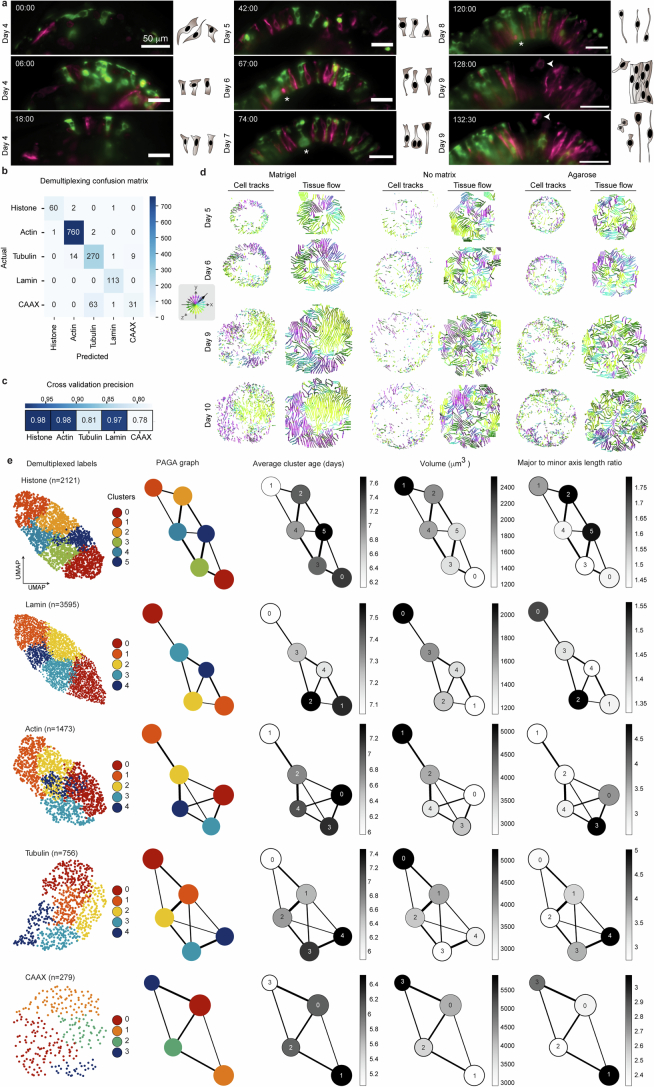
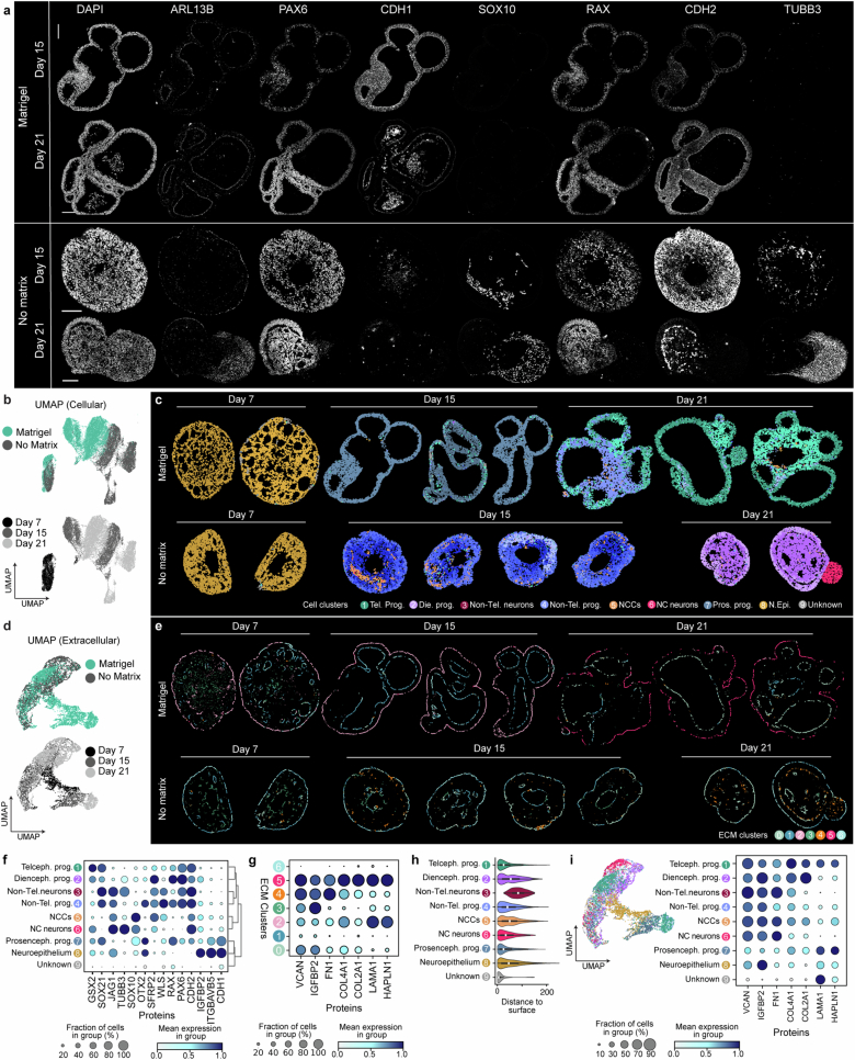
Brain organoids enable the mechanistic study of human brain development and provide opportunities to explore self-organization in unconstrained developmental systems^1-3. Here we establish long-term, live light-sheet microscopy on unguided brain organoids generated from fluorescently labelled human induced pluripotent stem cells, which enables tracking of tissue morphology, cell behaviours and subcellular features over weeks of organoid development⁴. We provide a novel dual-channel, multi-mosaic and multi-protein labelling strategy combined with a computational demultiplexing approach to enable simultaneous quantification of distinct subcellular features during organoid development. We track actin, tubulin, plasma membrane, nucleus and nuclear envelope dynamics, and quantify cell morphometric and alignment changes during tissue-state transitions including neuroepithelial induction, maturation, lumenization and brain regionalization. On the basis of imaging and single-cell transcriptome modalities, we find that lumenal expansion and cell morphotype composition within the developing neuroepithelium are associated with modulation of gene expression programs involving extracellular matrix pathway regulators and mechanosensing. We show that an extrinsically provided matrix enhances lumen expansion as well as telencephalon formation, and unguided organoids grown in the absence of an extrinsic matrix have altered morphologies with increased neural crest and caudalized tissue identity. Matrix-induced regional guidance and lumen morphogenesis are linked to the WNT and Hippo (YAP1) signalling pathways, including spatially restricted induction of the WNT ligand secretion mediator (WLS) that marks the earliest emergence of non-telencephalic brain regions. Together, our work provides an inroad into studying human brain morphodynamics and supports a view that matrix-linked mechanosensing dynamics have a central role during brain regionalization.

Fig. 1. Long-term live imaging of sparse and multi-mosaic fluorescently labelled brain organoids.

a, Schematic of the mosaic fluorescent organoid protocol and light-sheet image acquisition setup. EB, Embryoid body. b, UMAP embedding of organoid time-course scRNA-seq data with cells coloured by cluster and labelled by cell population (left) or time point (right). See Methods for cell numbers (n) at each timepoint. c, Stacked barplot showing the proportion of each cell population per time point. d, Feature plots showing normalized expression of representative marker genes. e, Maximum intensity projection image at 75 h of imaging from a 188-h imaging experiment. Organoids contain five different cell lines that contain stable genetic tagging of proteins with red or green fluorescent protein (RFP and GFP, respectively), as well as unlabelled cells. Scale bar, 100 µm. n = 16 organoids, imaged together. f, Organoid cross-section (84 h) showing nuclear membrane (lamin, RFP in magenta), plasma membrane label (CAAX, RFP in magenta), actin (GFP in green), tubulin (RFP in magenta) and nuclei (histone, GFP in green). Scale bar, 50 µm. g, Images of one organoid at different time points from a timecourse imaging experiment showing the maximum intensity projection (left) and cross-section (right). Scale bar, 100 µm. h, Cross-sections of an organoid showing lumen formation and fusion over time (hours). Dashed lines outline the lumen. Scale bar, 100 µm. 16 organoids, imaged together. i, 3D-rendered organoid showing segmented lumen and organoid epithelium masks. j, Graph showing total organoid volume measured per day from day 4 to day 9. k, Graph showing total volume of all lumen over time. l, Graph showing change in total number of segmented lumen over time. The dashed vertical line indicates the peak lumen number. The grey shading indicates standard deviation and the centre line denotes the mean (j–l). The dashed vertical lines in j and k denote the minimum (first line) and maximum (second line) of the lumen volume (%).

Fig. 2. Extrinsic ECM affects brain organoid morphogenesis.

a, UMAP embedding of scRNA-seq data with cells coloured by diffusion component ranking. b, Density plots showing cell distributions arranged in a pseudotime prediction (diffusion component 1 (DC1)) for time point (left) and cell type (right) labels. c, Heatmap showing normalized gene expression over DC1 ranking. d, Top DAVID Gene Ontology analysis terms calculated for genes that change over pseudotime from day 5 to day 11. A Fisher’s exact test was used to assess the significance of enrichment. e, Feature plots showing normalized expression of example ECM-related genes that show an increase in expression over time. f, Schematic representation of the extracellular microenvironment and the corresponding brightfield image for organoids grown with Matrigel (extrinsic ECM), without any external embedding (no-matrix) and with a low-melting agarose embedding (diffusion barrier). N = 3, n = 4 organoids. Scale bars, 100 µm. g, Images show cross-sections of sparse and multi-mosaic organoids containing cells labelled with nuclear membrane (lamin, RFP in orange), actin (GFP in cyan), tubulin (RFP in orange) and unlabelled cells from a light-sheet imaging experiment where organoids were embedded in Matrigel (n = 4), no-matrix (n = 8) or 0.6% agarose diffusion barrier (n = 4). The dashed lines outline the lumen. Scale bars, 100 µm. h, 3D renderings of segmented lumen in the organoids shown in panel g, colour coded for lumen axis measurements. i, Graphs showing total lumen number (top) measured per day from day 4 to day 9 for all imaged organoids, and total volume of all lumen (bottom) over time. j, Graph showing the number of lumen fusions over time. The shading indicates standard deviation and the centre line denotes the mean (i,j).

Fig. 3. Cell and nucleus morphology transitions using demultiplexed mosaic cellular labels.

a, Image analysis pipeline used for cell segmentation, demultiplexing and downstream analysis of mosaic cell labels. b, Maximum intensity projection image of an organoid at day 6 (left) showing dual-channel data (lamin, CAAX, tubulin (RFP, magenta), and actin, histone (GFP, green). Right: Corresponding demultiplexed images labelled with nuclear membrane (lamin, red), plasma membrane (CAAX, orange), actin (blue), tubulin (magenta) and nuclei (histone, green). Scale bar, 100 µm. c, Maximum intensity projection of demultiplexed image (lamin in red; CAAX in orange; actin in blue; tubulin in magenta; and histone in green). Scale bar, 100 µm. d, 4D cell tracks and tissue flows (averaged from tracks up to the last 24 h) during lumen expansion measured for all segmented actin-labelled cells from Matrigel, no-matrix and agarose conditions. The inset shows the colour key for arrow movements in 3D: white is towards the imaging objective and black is away from the imaging objective. e, Violin plot showing cell movements from the organoid centre towards the organoid surface (+1); n = 256 for Matrigel, 191 for no-matrix and 279 for agarose. f, PAGA initialized UMAP embeddings of all demultiplexed labels based on morphometric feature extraction. g, PAGA-initialized UMAP embeddings showing change in axis length for actin, tubulin and CAAX labels and change in nuclei volume measured using histone and lamin segmentations. PAGA plots show change in average cluster age (days), node size indicates the number of cells within one cluster, and edge width reflects the strength of connection between two clusters. h, PAGA-initialized UMAP embeddings and PAGA plots showing cell morphotype clusters using cells segmented from Matrigel, no-matrix and agarose conditions. The plots are based on morphometric measurements extracted for all segmented cells (actin). i, PAGA-initialized UMAP embeddings show a change in axis ratio of cells over time overlaid with average cluster age shown using PAGA plots. PAGA plots are colour coded based on the average age of the cluster from light grey to black. j, Heatmap showing example morphometric measurements for each morphotype cluster that are used to generate PAGA-initialized UMAP in panels h,i. k, Spatial distributions of actin-labelled cells in organoids showing cells coloured by their morphotype clusters. l, Example cells (actin) belonging to each of the morphotype clusters. m, Stacked barplots showing the proportion of cells in individual actin morphotype clusters in Matrigel, no-matrix and agarose conditions. n, All cells (actin) coloured by their alignment index (absolute cosine of the angle to the nearest organoid surface normal). Scale is from 0 to 1, with 1 (red) corresponding to cells that align perpendicular to the organoid surface. o, Violin plot showing the cell alignment (actin) values across all segmented cells from day 4 to day 12 for all three conditions. The boxes of the violin plots show the interquartile range, the line at the centre is the median and the whiskers extend to the data range excluding outliers (e,o).

Fig. 4. Multiplexed immunohistochemistry (4i) reveals spatial region emergence in organoid development.

a, Overview of the 4i data acquisition pipeline. Organoids from a timecourse were fixed and sectioned followed by mounting on a glass coverslip. b, Image showing an example organoid section with segmented compartments (extracellular, cytoplasmic and nuclear) used for downstream quantitative analysis. c, Selected images showing protein stainings on day 21 on organoid slices in Matrigel (n = 4) and no-matrix (n = 3) conditions. d, UMAP embedding based on the combined cellular (nuclear + cytoplasmic) protein expression, with each dot representing a cell, clustered and annotated as distinct cell types. e, Example organoids (day 21) from each condition (Matrigel and no-matrix) with cell clusters projected back to the image. f, UMAP embedding based on the combined protein expression in the extracellular compartment showing individual clusters. g, Example organoids (day 21) from each condition (Matrigel and no-matrix) with extracellular cell clusters projected back to the image. h, Stacked barplot showing the cluster proportion of each cell population from all days in Matrigel and no-matrix conditions. *P < 0.05, calculated using a Fisher's exact test (two-sided) between the cluster proportions of the conditions corrected for multiple testing using the Benjamini–Hochberg method. For P values, see Supplementary Table 13. i, Stacked barplot showing the ECM cluster proportion per cell population. The violin plots show the major axis of the lumen that have been assigned to each cell cluster. Dienceph, diencephalic; NC, neural crest; NCC, neural crest cell; prog., progenitor; prosenceph., prosencephalic; tel., telencephalic. j, Violin plot showing the protein expression in extracellular and cellular compartments in Matrigel and no-matrix conditions. *P < 0.05, calculated using a one-way analysis of variance (ANOVA) across the timepoints for a condition corrected for multiple testing using the Benjamini–Hochberg method. n = 5,137 for Matrigel and n = 3,958 for no-matrix for the extracellular quantifications, and n = 17,140 for Matrigel and n = 16,007 for no-matrix for the cytoplasmic quantifications. The boxes of the violin plots show the interquartile range, the line at the centre is the median and the whiskers extend to the data range excluding outliers (i,j). For P values, see Supplementary Table 13. Scale bars, 100 µm (all panels).

Fig. 5. YAP1 mechanotransduction-mediated WLS activation.

a, Images show cross-sections of organoids stained with antibodies labelling YAP1 (day 16) and WLS (day 15) from Matrigel and no-matrix conditions. Scale bars, 100 µm. b, Violin plots showing protein expression distribution of nuclear YAP1 (day 16) and cytoplasmic WLS (day 15) from Matrigel and no-matrix conditions. *P < 0.05, calculated using a Wilcoxon rank-sum test (two-sided) between conditions corrected for multiple testing using the Benjamini–Hochberg method. The boxes of the violin plots show the interquartile range, the line at the centre is the median and the whiskers extend to the data range excluding outliers. For P values, see Supplementary Table 13. c, Schematic showing the developing brain with distinct regions along the rostrocaudal axis: prosencephalon (telencephalon (Tel.) + diencephalon (Die.)), mesencephalon (Mes.) and rhombencephalon (Rh.). The dotted lines show coronal sections to illustrate lumen (brain ventricle) size differences. A schematic summarizing the morphological distinctions between Matrigel and no-matrix organoids with corresponding YAP1 and WLS expression differences is also shown (right). d, Signal tracks of bulk CUT&Tag sequencing data showing the enrichment intensity of YAP1 binding to the WLS gene, profiled with two different YAP1 antibodies. Tracks are shown for IgG and Tn5 control and the repressive and active marks profiled with H3K27me3, H3K4me3 and H3K9ac antibodies. Chr. 1, chromosome 1. e, Schematic of the light-sheet imaging and scRNA-seq experiment with control and YAP1 activator-treated organoids (top). EBs were cultured in NIM with Matrigel embedding on day 4. YAP1 activator (Py-60) or DMSO (control) was added to the imaging sub-chamber on day 5 or day 7. Imaging was terminated on day 10, and corresponding organoids from all three conditions were profiled with scRNA-seq on day 10. UMAP embeddings of scRNA-seq data from day 10 organoids in control and YAP1 treatment conditions are also shown (bottom left). A stacked barplot showing the cluster proportion of each cell population is also shown (bottom right). *P < 0.05, calculated using a Fisher’s exact test between the cluster proportions of the control and day 5-treated or day 7-treated conditions corrected for multiple testing using the Benjamini–Hochberg method. For P values, see Supplementary Table 13. The number of cells recovered after pre-processing of the scRNA-seq experiment: n = 2,085 for control, n = 763 for Py-60 on day 5 and n = 1,955 for Py-60 on day 7. f, Dotplot showing average expression and percentage of cells expressing selected regional marker genes per cell population. g, Maximum intensity projections (left) and cross-sections (right) at day 8, showing control organoids and YAP1 activator (given on day 5) treated organoids imaged with light-sheet microscopy. Sparse and multi-mosaic organoids contain cells labelled with nuclear membrane (lamin, RFP in orange), actin (GFP in cyan) and tubulin (RFP in orange) and unlabelled cells. Scale bars, 100 µm. Organoids imaged per condition, n = 4. h, Schematic of the scRNA-seq experiment with organoids generated from control and WLS-knockout (WLS-KO) iPS cell lines with five treatments. EBs were cultured in Matrigel or no-matrix conditions starting at day 4. WNT (CHIR99021) or YAP1 (Py-60) activators were added to a subset of organoids cultured with Matrigel from day 10 to day 12 and day 10 to day 16, respectively. Organoids were hashed and profiled with scRNA-seq on day 55. i, UMAP embeddings of scRNA-seq data coloured by cell population (top), genetic status (bottom left) or condition (bottom right). Mes./rhomb., mesencephalon or rhombencephalon. j, Stacked barplot showing the cluster proportion of each cell population in the different treatment conditions. k, Dotplot showing the average expression and the percentage of cells expressing selected regional marker genes per cell populations.

Extended Data Fig. 1. Protocol development for organoids compatible with long-term live light sheet imaging.

a) Schematic of the protocol developed in this study (Protocol I) and a previous protocol to develop multi-region brain organoids (Protocol II)^,. b) Comparison of organoid size at day 4 post aggregation at two cell seeding concentrations. Scale Bar is 500 micrometers. c) Brightfield images showing organoid growth from day 8–11 in the two different protocols. N = 3, n > 3. Scale Bar is 500 micrometers. d) Heatmap showing normalized marker gene expression grouped per cluster of organoid time-course scRNA-seq data shown in Fig. 1b. e,f) Images of example organoids stained with fluorescence in situ hybridization chain reaction (HCR) showing regionalized expression of marker genes in false color, merged using Fiji. Three organoids were used for staining in each case and the n indicates the number of organoids imaged. Organoids were stained whole-mount and images were acquired as z-stacks. Selected cross-sections after reorientation of the acquired volume are shown for each organoid. e) Day 11 (top n = 1), (bottom n = 3). f) Day 15 top left, n = 2, top right n = 3, middle left n = 1, middle right n = 3, bottom left n = 3. Scale, 250 micrometers in all images.

Extended Data Fig. 2. Long-term live imaging of fluorescent brain organoids.

a) Photographs of the sample holding chamber with four separated sub-chambers each containing four microwells, for growing and imaging organoids with sixteen different organoids arranged one per microwell n = 16 organoids. b) Schematic overview of tiled image acquisition and example images showing two timepoints, before and after tiled acquisition and image fusion. Scale Bar is 100 micrometers. Time is in hours. n = 16 organoids. c) Cross section images (day 7) from 16 simultaneously imaged organoids, generated with cells lines labeled with nuclear membrane (lamin, RFP, magenta), plasma membrane (CAAX, RFP, magenta), actin (GFP, green), tubulin (RFP, magenta), and nuclei (histone, GFP, green) and unlabeled WTC-11. d) Images showing cross section (z-plane) and orthogonal views (y-plane, x-plane) of one organoid from a timecourse lightsheet imaging experiment shown in c. Scale Bar is 100 micrometers. Time is in hours. e) Maximum intensity projections from a 2-week imaging acquisition of a mosaic organoid (histone, GFP, green; CAAX, RFP, magenta), unlabeled WTC-11). Scale Bar is 500 micrometers. Time is in hours. n = 16 organoids. f) Images from a 3-week continuous imaging experiment using a NKX2-1:GFP reporter line. The organoids were given SHH morphogen treatment to induce ventral telencephalic patterning of the organoids. Images are false-colored with the green-fire-blue LUT. Scale Bar is 100 micrometers. Time is in hours. n = 4 organoids.

Extended Data Fig. 3. Lightsheet imaging and lumen segmentations to track tissue morphodynamics in organoid development.

a) 2D cross sections from a time course lightsheet movie showing lumen development. Organoids were generated from 100% single label iPSC lines (histone2B-mEGFP mEGFP-beta-actin, mTagRFP–T–CAAX, mTagRFP–T-tubulin-alpha1b and mTagRFP–T-laminB1). Scale, 100 micrometers. Time is in hours. Three organoids were imaged for each label (n = 3). b) 2D cross sections from 3D imaged and segmented organoids shown in a, with organoid epithelium (gray) and segmented lumen (red) on day 9. Scale Bar is 100 micrometers. c) Violin plots showing 3D lumen volumes of organoids shown in a, over time. d) Violin plots showing lumen volumes on day 9, with horizontal bars indicating pairwise Wilcoxon rank sum test corrected for multiple testing using the Bonferroni method. P-values were > 0.5 for all comparisons. n.s. = not significant. e) Violin plots showing the major axis lengths of lumen over time. f) Violin plots showing the major axis lengths of lumen on day 9, with horizontal bars indicating Wilcoxon rank sum test corrected for multiple testing using the Bonferroni method. P-values were > 0.5 for all comparisons. n.s. = not significant. For p-values (d,f) see Supplementary Table 13. (c-f) The boxes of the violin plots show the interquartile range, the line at the center is the median and the whiskers extend to the data range excluding outliers.

Extended Data Fig. 4. Lumen segmentations to track organoid and lumen morphodynamics in organoid development.

a) 2D cross sections showing organoid epithelium (gray) and segmented lumen (red) from day 4–7. Scale, 500 micrometers. Time is in hours. All 16 organoids were imaged in one experiment. b) 3D renderings of segmented lumen for the corresponding organoids shown in a. Time is in hours. c) Plot shows individual lumen volumes over time, from day 4 to day 9, of all segmented lumen from organoids shown in a and b. d) 3D renderings of lumen segmentations and tracking. Lumens from the same track show the same color. 16 organoids were imaged in one experiment with 4 different organoids in matrigel condition, 8 organoids from no-matrix condition and 4 organoids for diffusion barrier condition. Time is in hours. e-h) Graphs showing total organoid volume (e), epithelium volume (f), individual lumen volumes (g) and mean major axis length measurements (h) of all segmented lumen for all imaged organoids in d. Error bars indicate standard deviation and the center line indicates the mean (e, f, h). Total imaged organoids used for measurements: Matrigel (n = 4), no-matrix (n = 8) and Diffusion barrier (n = 4). i) 3D renderings of segmented lumen in organoids shown in Fig. 2g, color coded for lumen volume. j) 3D renderings of segmented lumen in organoids shown in Fig. 2g, showing a timecourse of lumen development in Matrigel, no-matrix and agarose conditions. Lumen were segmented and tracked overtime. Color shows the hours from the last fusion event with yellow indicating the just fused lumen.

Extended Data Fig. 5. Mechanical and molecular differences in embedding matrix impact lumen morphogenesis and gene expression in developing organoids.

a) 2D cross sections from a time course lightsheet movie showing lumen development. Organoids were generated from 100% single label iPSC line (mTagRFP–T-tubulin-alpha1b) and embedded in 0.3% Agarose. Scale, 100 micrometers. Time is in hours. b,c) Graphs showing % lumen volumes and number of lumen (normalised to organoid volume) of organoids shown in a, compared with multimosaic organoids (WTC-11, nuclear membrane (lamin, RFP, magenta), actin (GFP, green), tubulin (RFP, magenta)) embedded in 0.6% agarose shown in Fig. 2f. A single time point per day was segmented and used for quantifications. Error bars indicate standard deviation and the center line the mean, n = 4. d) 2D cross sections from a time course lightsheet movie showing lumen development in multi-mosaic labelled organoids (WTC-11, nuclear membrane (lamin, RFP, magenta), actin (GFP, green), tubulin (RFP, magenta)) that were embedded in PEG-RDG (control), PEG-LAM and PEG-GFOGER with controlled stiffness. n = 4 organoids for each condition. Scale, 100 micrometers. Time is in hours. e) 2D cross sections from organoids that were imaged on Day 8, using lightsheet showing lumen development in multi-mosaic labelled organoids (WTC-11, nuclear membrane (lamin, RFP, magenta), actin (GFP, green), tubulin (RFP, magenta)) that were embedded in PEG-RDG (control), PEG-LAM and PEG-GFOGER with controlled stiffness. 16 organoids from each condition were embedded in the same chamber and imaged. f) Graphs showing number of lumen and normalized lumen volumes of organoids shown in d. A single time point per day was segmented and used for quantifications. Error bars indicate standard deviation and the center line the mean, n = 4 for each condition. g,h) RNA sequencing analysis of organoids shown in e and used for a bulk RNAseq experiment. The bar plot shows the Spearman correlation coefficients between logFC of each PEG condition with PEG-RDG, and logFC of Matrigel relative to no-ECM, across highly variable genes in the samples (g). Heatmap showing genes upregulated in PEG-LAM, PEG-LAM-GFOGER and PEG-GFOGER compared with PEG-RDG and upregulated in Matrigel compared with no-matrix on day 8 and day 13 (h).

Extended Data Fig. 6. Demultiplexed labels reveal cellular morphodynamics.

a) Cross-sections showing cell shape transitions from embryoid bodies to different stages of neuroepithelium formation and maturation in organoids from day 4 to day 9. Illustrations show different cell shapes seen in the cross-section images. Organoids are labeled with nuclear membrane (lamin, RFP, magenta), plasma membrane label (CAAX, RFP, magenta), actin (GFP, green), tubulin (RFP, magenta), and nuclei (histone, GFP, green). Asterisks mark cell division events seen in tubulin (magenta) and actin(green) labels. Arrowheads mark cell divisions on the basal surface of the organoids. Time is in hours. Scale, 50 micrometers. n = 16 organoids. b) Confusion matrix showing total number of demultiplexed cells assigned to each label and misclassifications between labels. c) The marker specific precision for demultiplexed labeling. d) 4D cell tracks and consequent tissue flows (averaged from tracks up to the last 24 h) for all segmented actin cells from Matrigel, no-matrix, and agarose conditions. e) UMAP embeddings and PAGA plots showing cell morphotype clusters of all 5 demultiplexed labels based on morphometric feature extraction. The PAGA plots per label show average cluster age, the change in nuclei volume and the change in axis length measured over time across all segmented cells. n number indicates the total number of cells per label from all timepoints.

Extended Data Fig. 7. Demultiplexed labels reveal cellular morphodynamics in matrix perturbations.

a) Demultiplexed images (lamin, yellow; actin, cyan; tubulin, magenta) of example organoids that were embedded with Matrigel, given no-matrix or embedded in agarose and imaged from day 4–12 in a light sheet microscope. Scale, 500 micrometers. b) UMAP embeddings showing clusters in lamin and tubulin labels based on morphometric feature extraction, change in axis length and volume measured using cell segmentations. PAGA plots show change in average cluster age (days). c) Extended heatmap from Fig. 3j, showing example morphometric measurements used for generating the PAGA derived UMAP shown in Fig. 3i. Day corresponds to real time and dpt_pseudotime is pseudotemporal ordering of cells in every morphotype cluster. d) Box plot showing axis length ratio per day in actin labeled cells across the 3 conditions, with the median shown, where the boxes show the quartiles of the measurement and the whiskers, the 1.5 IQRs of the lower and upper quartile. e) PAGA heatmap showing actin morphometric measurements derived from high resolution clustering. Day corresponds to real time and dpt_pseudotime is pseudotemporal ordering of cells in every morphotype cluster. f) PAGA plots showing high resolution clustering, volume, axis length ratio and average cluster age in days. g) Images segmented show cells (lamin, actin, tubulin) colored by their alignment index (absolute cosine of the angle to the nearest organoid surface normal) in all three conditions over time. Red colors indicate higher alignment (perpendicularity) to the cell surface. h) Violin plot showing the cell alignment values across all segmented cells (actin) from day 4 to day 12 for all three matrix conditions. The boxes of the violin plots show the interquartile range, the line at the center is the median and the whiskers extend to the data range excluding outliers. The n numbers (number of cells from all organoids per condition) are (Matrigel: day 4 to 12, n = 206, 462, 796, 865, 839, 871, 946, 778, 403), (No-matrix: day 4 to 12, n = 320, 521, 810, 732, 698, 791, 926, 872, 659), (agarose: day 4 to 12, n = 286, 454, 481, 547, 699, 684, 678, 557, 315). i) Line plot showing the change in Shannon index between the three conditions based on change in the number of cells per cluster over time (organoids: Matrigel (n = 3), no-matrix (n = 3) and agarose (n = 3)) shown in Fig. 3m, with the error bars being the 95 percent confidence intervals and the center line the mean based on a bootstrapping analysis with 1000 repeats.

Extended Data Fig. 8. Multiplexed immunohistochemistry on matrix perturbations.

a) Selected images show protein stainings on day 15 and 21 on organoid slices in Matrigel and no-matrix conditions, n numbers are added to c. b) UMAP embedding of multiplexed immunohistochemistry data (4i) based on cellular expression of proteins (Fig. 4d), with cells colored by treatment (Matrigel, no-matrix) and time (day 7, 15, 21). c) Spatial mapping of cell clusters in each organoid used for the combined analysis. The cell clusters are projected back to the original images from Matrigel and no-matrix conditions over the time course (day 7, 15, 21). Matrigel: day 7 n = 2, day 15 n = 3 and day 21 n = 4. No-matrix: day 7 n = 2, day 15 n = 4 and day 21 n = 3. d) UMAP embedding of multiplexed immunohistochemistry data (4i) based on the protein expression in the extracellular compartment of cells, with cells colored by treatment (Matrigel, no-matrix) and time (day 7, 15, 21). e) Spatial mapping of ECM clusters in each organoid used for the combined analysis. The ECM clusters are projected back to the original images from Matrigel and no-matrix conditions over the timecourse (day 7, 15, 21). f) Dotplot showing average expression and percentage of cells expressing selected regional marker proteins per cluster in b. g) Dotplot showing average expression and percentage of cells expressing ECM proteins per cluster in d. h) Violin plots showing the distance of each cell cluster from the organoid surface. The boxes in the violin plots show the interquartile range, with the line at the center as the median and the whiskers extending to the data range excluding outliers. i) UMAP embedding of multiplexed immunohistochemistry data (4i) based on the protein expression in the extracellular compartment of cells (shown in d, Fig. 4f), showing the distribution of cellular clusters shown in c and Fig. 4d. Right: Dotplot showing average expression and percentage of cells expressing ECM proteins in each cellular cluster. Scale, 100 micrometers in all images.

Extended Data Fig. 9. Multiplexed immunohistochemistry on matrix perturbations.

a) Selected images show stainings of ECM proteins on day 15 and 21 on organoid slices in Matrigel and no-matrix conditions. b) Images show cross sections from an immunohistochemistry experiment on organoids (day 15) grown with Matrigel (n = 4) or with no-matrix (n = 4) and stained to show nuclei (DAPI), COL4A1 and CDH2. Scale Bar is 100 micrometers in all images. c) Example organoids from each condition (Matrigel, no-matrix) on day 15 and day 21 colored by cell clusters projected back to the image. Boxes highlight the luminal region from insets are shown in d. d) Images show lumen in organoids shown in c with ARL13B and LAMA1 protein expression marking neuroepithelium polarity. e,f) Images show protein stainings on organoid slices that were embedded in 0.6% agarose, fixed and stained in a 4i experiment. Day 7 (n = 2) and day 11 (n = 3). Images show polarity marker proteins (e) and ECM proteins (f). Scale, 100 micrometers in all images.

Extended Data Fig. 10. Matrix impacts organoid patterning and regionalization.

a-b) UMAP embedding of scRNA-seq data with cells colored by condition (a) and cell population (b). Stacked barplot shows cluster proportion per condition. Abbreviations: Non-telen. = Non telencephalic, PSCs = Pluripotent stem cells. A star indicates p < 0.05, calculated using a Fisher’s exact test between the cluster proportions of Matrigel and no-matrix or agarose conditions, corrected for multiple testing using the Benjamini-Hochberg method. For p-values see Supplementary Table 13. c) Volcano plot highlights differentially expressed genes between Matrigel and no-matrix conditions calculated using a non-parametric Wilcoxon Rank Sum test with p-value cutoff using adjusted p-value. The p-value adjustment was performed using Bonferroni correction based on the total number of genes in the dataset. Positive and negative log fold change indicates genes with higher expression in Matrigel or higher expression in no-matrix conditions, respectively. GO/KEGG terms enriched for genes differentially upregulated between Matrigel (right) and no-matrix (left) conditions are shown. Heatmaps show average gene expression of selected differentially expressed genes in different regions of the human fetal brain tissue from 5-14 post-conceptional weeks. d) Cross sections from a whole mount fluorescence in situ hybridization chain reaction (HCR) staining for selected differentially expressed genes between Matrigel and no-matrix conditions. Scale, 100 micrometers. n = 3. e) Violin plots showing the total protein expression in Matrigel and no-matrix organoids over time and calculated from the 4i experiment shown in Fig. 4 and Extended Data Figs. 8 and 9. The boxes of the violin plots show the interquartile range, the line at the center is the median and the whiskers extend to the data range excluding outliers. A star indicates p < 0.05, calculated using a Wilcoxon rank sum test (two-sided) between conditions corrected for multiple testing using the Benjamini-Hochberg method. For p-values see Supplementary Table 13. n = 5289 (Day 7), n = 11690 (Day 15), n = 16168 (Day 21).

Extended Data Fig. 11. Matrigel influences organoid regional patterning.

a) Overview of the protocol used to generate organoids to test the influence of matrix on brain organoids development (Cerebral organoid, Protocol II). b) Time-course images of organoids generated from mTagRFP–T-Tubulin-alpha1b iPSC line, showing merged brightfield and RFP expression in the presence (n = 4) and absence (n = 2) of Matrigel. Imaging was done with a widefield Nikon Ti2 microscope. c) UMAP embeddings of scRNA-seq data performed at day 16 with cells labeled by treatment (left) or colored by cluster and labeled by cell population (right). d) Feature plots showing normalized expression of selected marker genes. e) barplot showing cluster proportions of the cell populations in Matrigel and no-matrix organoids. f) Volcano plot showing differentially expressed genes upregulated in Matrigel (right) and upregulated in no-matrix conditions (left), calculated using a non-parametric Wilcoxon Rank Sum test with p-value cutoff using adjusted p-value. The p-value adjustment was performed using Bonferroni correction based on the total number of genes in the dataset. g-k) Images show example organoids stained whole-mount with fluorescence in situ hybridization chain reaction (HCR) showing regionalized expression of marker genes (false color, merged using Fiji) between organoids grown with Matrigel or with no-matrix. Three organoids were used for staining in each case. The n indicates the number of organoids imaged. g) Images show maximum intensity projections of organoids treated with Matrigel (top, n = 2) and or with no-matrix (bottom, n = 1) on day 15. Organoids were generated with protocol II, shown in a. Scale, 100 micrometers. h-k) Cross section images of HCR stainings. h) Day 7, Matrigel n = 1 and no-matrix n = 2. i) Day 11, n = 3 for both. j) Day 15 n = 3 for both. k) Day 15 no-matrix n = 2 and Matrigel n = 3. Organoids were generated with protocol shown in Fig. 1a. Scale, 250 micrometers.

Extended Data Fig. 12. YAP1 and WLS influence organoid patterning.

a) Violin plots showing the expression of nuclear YAP1 in organoids over time (immunohistochemical staining quantification). (Matrigel number of nuclei (days 7,11,16): n = 4631, 5104, 13824, no-matrix (days 7,11,16): n = 3390, 5023, 11025). b) Barplot shows relative WLS expression in no-matrix organoids on day 15 measured using qPCR, averaged from 3 replicates, N = 1. Organoids were treated with YAP1 activators (TRULI, GA-017, Py-60) and inhibitor (TED-34) on day 10. c) Brightfield images at day 13, showing a control organoid (n = 5) and an organoid cultured with YAP1 activator (10 µM Py-60) together with Matrigel (n = 13) from day 10 onwards. Organoid protocol is shown in Extended Data Fig. 11a. Scale, 100 micrometers. d) UMAP embedding of scRNA-seq data from 16-day old organoids with cells colored by treatment (top) and cluster and labeled by cell population (bottom). Abbreviations: N.ecto = neuroectoderm, NCC = neural crest cells and EMT = epithelial-to-mesenchymal transition. e) Feature Plots showing normalized expression of marker genes. f) Stacked barplot showing the proportion of each cell population in control and YAP1 activator treatment. g) Dotplot showing average expression and percentage of cells expressing selected regional marker genes used for annotating the cell populations shown in d. h) Maximum intensity projections and cross-section images at day 8 showing control and YAP1 activator (given on day 7) treated organoids imaged with lightsheet microscopy. Sparse and multi-mosaic organoids contain cells labeled with nuclear membrane (lamin, RFP, orange), actin (GFP, cyan) and tubulin (RFP, orange) and unlabeled cells. Scale, 100 micrometers. n = 4. i,j) Snapshots of CRISPResso2 readout showing quantification of editing frequency as determined by the percentage and number of reads showing unmodified and modified alleles for the control (unedited) and WLS-KO cell lines. k) Brightfield images showing 54-day old organoids generated from control and WLS-KO cell lines and given different treatments. The organoids were used for single-cell RNAseq on day 55 (Fig. 5h–k). Scale, 500 micrometers. n = 12 for Matrigel and no-matrix, n = 8 for DMSO control, Py-60 and CHIR99021 treatments l,m) Volcano plot highlights differentially expressed genes between Matrigel and no-matrix conditions from organoids treated with Chiron (l) or Py-60 (m). Positive and negative log fold change indicates genes with higher expression in Matrigel or higher expression in no-matrix conditions, respectively. The differential gene expression was calculated using a non-parametric Wilcoxon Rank Sum test with p-value cutoff using adjusted p-value. The p-value adjustment was performed using Bonferroni correction based on the total number of genes in the dataset.

References

1. Eiraku, M. et al. Self-organized formation of polarized cortical tissues from ESCs and its active manipulation by extrinsic signals. Cell Stem Cell3, 519–532 (2008). - PubMed
1. Lancaster, M. A. et al. Cerebral organoids model human brain development and microcephaly. Nature501, 373–379 (2013). - PMC - PubMed
1. Mariani, J. et al. Modeling human cortical development in vitro using induced pluripotent stem cells. Proc. Natl Acad. Sci. USA109, 12770–12775 (2012). - PMC - PubMed
1. Huisken, J., Swoger, J., Del Bene, F., Wittbrodt, J. & Stelzer, E. H. K. Optical sectioning deep inside live embryos by selective plane illumination microscopy. Science305, 1007–1009 (2004). - PubMed
1. Camp, J. G. et al. Human cerebral organoids recapitulate gene expression programs of fetal neocortex development. Proc. Natl Acad. Sci. USA112, 15672–15677 (2015). - PMC - PubMed
MeSH terms
Substances
LinkOut - more resources