Optimizing genomic diversity assessments for conservation of Bromus auleticus (Trinius ex Nees) using individual and pooled sequencing

Abstract

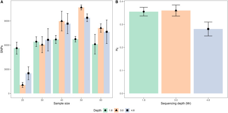
Bromus auleticus, a valuable forage grass native to the Pampa biome, is currently undergoing genetic erosion. Therefore, it is essential to assess appropriate methodologies for developing population genomic studies that will contribute to the conservation of this genetic resource. In this study, we evaluated five accessions using two genotyping strategies: individual sequencing (ind-seq) and pooled sequencing (pool-seq). To assess methodologies effectiveness, the correlation between allele frequencies calculated using each approach was investigated, as well as genetic diversity and population structure. These comparisons explicitly accounted for the potential effects of factors such as sample size, missing data, sequencing depth, and minor allele frequencies. The highest values of frequencies concordance and percentage of SNPs in common between ind-seq and pool-seq were achieved using a sample size of 30-60 plants per accession. These values were obtained with a maximum missing data threshold of 10% and a less strict minimum allele frequency threshold for pool-seq (0.01) compared to ind-seq (0.05). Pool-seq required a higher sequencing depth per accession (4.8 million reads) compared to ind-seq (0.9 million reads) to achieve similar allele frequencies. Pools of 50 individuals yielded the highest number of polymorphic sites, averaging over 9,000 per accession at a sequencing depth of 4.8 Mr. Under these conditions, pool-seq consistently resulted in an average of 0.09 higher expected heterozygosity and a 0.24 lower allelic richness compared to ind-seq in all accessions. Population structure inferred with both methodologies confirmed the outcrossing nature of B. auleticus and aligned with the geographical origin of each accession. The average inbreeding coefficient of 0.2 evidence inbreeding, which highlights the importance of conservation efforts for this valuable plant genetic resource. Based on these findings, we propose two workflows for conducting population genomics studies on Bromus auleticus.

Fig 1. Geographical map of Uruguay showing the spatial distribution of the 82 accessions conserved in the INIA germplasm bank.

The purple diamonds indicate the five accessions evaluated in this study. Black circles represent the 77 accessions pending genomic evaluation. The map includes ecoregions according to the classification framework established by Brazeiro et al. (2012) [51]. The colour scheme is delineated in the accompanying legend. The graph was generated using the “ggplot2” package in R [53].

Fig 2. Diagram illustrating the procedures and parameters analyzed, using one accession as an example.

(A.) Individual sequencing (ind-seq) (blue background) involved individual sample collection, unique barcoding, sequencing at 0.9 Mr depth, individual SNP calling, and analysis with dartR and Bio-R. (B.) Pooled sequencing (pool-seq) (pink background) involved two tissue replicates, two libraries per replicate, sequencing at two depths, pooled SNP calling, and analysis with Bio-R. (C.) Common SNP calling (orange background) is employed to compare allele frequencies between paired individuals and pools with the same sample size and missing data. The minimum allele frequency and sequencing depth used in the individual SNP dataset remained constant. They were compared with pooled datasets based on two MAF and three sequencing depths. See the step-by-step protocol for more details [54]. This diagram was created using Microsoft PowerPoint.

Fig 3. Effect of sample size (A, B) and missing data thresholds (MD) (C, D) on Representativity (%) and Concordance Correlation Coefficient (CCC).

Each data point represents the average Representativity or CCC for a single accession, with the color key provided in the legend. For each group, the black horizontal line indicates the means, while the vertical lines represent the standard error. The upper panels (A.) and (B.) illustrate the effect of different sample sizes (20, 30, 40, 50, 60) on Representativity and CCC, respectively. For the same metrics, the lower panels, (C.) and (D.), show the influence of MD thresholds (10, 20, 30, 40, 50, and 60%). Statistical differences between groups, as determined by Tukey’s test (p < 0.05), are indicated by different letters. Plots were generated using the “ggplot2” and “ggpubr” packages in R [53,70].

Fig 4. Effect of sequencing depth (Mr) (A, B) and minor allele frequency thresholds (MAF) (C, D) on Representativity (%) and Concordance Correlation Coefficient (CCC).

Each dot represents the average Representativity or CCC of an individual accession, with the color coding outlined in the accompanying legend. For each group, the black horizontal line indicates the mean values, while the vertical lines represent the standard deviation. Panels (A.) and (B.) show the effect of sequencing depth (1.8, 3.0, and 4.8 Mr) on Representativity and CCC, respectively. Panels (C.) and (D.) illustrate the effect of MAF thresholds (0.01 and 0.05) on Representativity and CCC, respectively. Statistical differences between groups, as determined by Tukey’s test (p < 0.05), are indicated by different letters. Plots were generated using the “ggplot2” and “ggpubr” packages in R [53,70].

Fig 5. Cumulative effect of optimized factors (Selected) on Representativity (%) and Concordance Correlation Coefficient (CCC).

“All” compresses the entire dataset from the S6 Table. The “Selected” dataset includes samples with a minimum size of 30 plants, a missing data (MD) threshold of 10%, a coverage depth of 4.8 Mr for pooled samples, and a MAF threshold of 0.01. Each point represents the average Representativity or CCC of a single accession, with the color coding detailed in the legend. For each group, the black horizontal line indicates the mean value, while the vertical line represents the standard deviation. (A.) Shows the effect of Selected data on Representativity. (B.) Displays the effect of Selected data on CCC. Statistical differences between groups, determined by Tukey’s test (p < 0.05), are indicated by different letters. Plots were generated using the “ggplot2” and “ggpubr” packages in R [53,70].

Fig 6. Effect of Sample size on Allele Richness (Ae).

Each dot represents a single accession, with the color coding detailed in the legend. For each group, the black horizontal line indicates the mean, while the vertical lines represent the standard deviation. Statistical differences between groups, determined by Tukey’s test (p < 0.05), are indicated by different letters. The plot was generated using the “ggplot2” package in R [53].

Fig 7. Effect of sample size and sequencing depth on single nucleotide polymorphisms (SNP) number and the influence of sequencing depth on Expected heterozygosity (H_E) with pool-seq dataset.

Panel (A.) presents the average number of SNPs (SNPs) across accessions, along with the corresponding standard deviation, stratified by sample size and sequencing depth. Panel (B.) illustrates the average expected heterozygosity and its standard deviation across all accessions at varying sequencing depths.

Fig 8. Boxplot illustrating influence of sequencing depth in

ΔH_E: H_E pool-seq – H_E ind-seq. Each dot represents a single accession, with color explained in the legend. The line inside each box represents the median, while the lower and upper box edges indicate the first and third quartiles, respectively. The whiskers extend from the box to the minimum and maximum values within 1.5 times the interquartile range from the first and third quartiles, respectively. Tukey’s test (p < 0.05) is indicated by letters statistical differences between groups. Plots were generated using the package “ggplot2” in R [53].

Fig 9. Multidimensional scaling (MDS) based on Roger’s distance.

(A.) MDS plot derived from individual sequencing (ind-seq) data using 50 individuals per accession and 2,124 single nucleotide polymorphisms (SNPs). (B.) MDS plot derived from pool sequencing (pool-seq) data using pools of 40, 50, and 60 plants with a sequencing depth of 4.8 Mr and 63,017 SNPs. Graphs were generated using the “plotly” library in Python [71].

Fig 10. Proposed workflows for analyzing genetic diversity in B. auleticus.

(A.) Ind-seq: individual sequencing approach. (B.) pool-seq: pooled sequencing workflow. The diagram outlines the number of samples, sequencing depth, R packages used, and the analyses proposed for each workflow. This diagram was created using Microsoft PowerPoint.

References

1. Bilenca D, Miñarro F. Identificación de áreas valiosas de pastizal (AVPs) en las pampas y campos de Argentina [Identification of valuable grassland areas (VPA) in the pampas and campos of Argentina]. Fundación Vida Silvestre Argentina, ed. Buenos Aires: Fundación Vida Silvestre Argentina; 2004. p. 353.
1. Olmos F. Bromus auleticus. First ed. Unidad de difusión e información tecnológica del INIA, ed. Montevideo: Unidad de difusión e información tecnológica del INIA; 1993. p. 30
1. Global core biodata resource. 2024. https://www.gbif.org/es/species/4107276. - PMC - PubMed
1. Artico LL, Mazzocato AC, Ferreira JL, Carvalho CR, Clarindo WR. Karyotype characterization and comparison of three hexaploid species of Bromus linnaeus, 1753 (Poaceae). Comp Cytogenet. 2017;11(2):213–23. doi: 10.3897/CompCytogen.v11i2.11572 - DOI - PMC - PubMed
1. Williams WM, Stewart AV, Williamson ML. Bromus. In: Kole C, ed. Wild crop relatives: genomic and breeding resources, millets and grasses. Berlin, Heidelberg: Springer-Verlag Berlin Heidelberg; 2011. p. 15–30.
LinkOut - more resources