Model-free photon analysis of diffusion-based single-molecule FRET experiments

Abstract

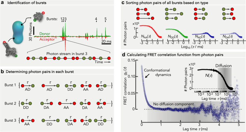
Photon-by-photon analysis tools for diffusion-based single-molecule Förster resonance energy transfer (smFRET) experiments often describe protein dynamics with Markov models. However, FRET efficiencies are only projections of the conformational space such that the measured dynamics can appear non-Markovian. Model-free methods to quantify FRET efficiency fluctuations would be desirable in this case. Here, we present such an approach. We determine FRET efficiency correlation functions free of artifacts from the finite length of photon trajectories or the diffusion of molecules through the confocal volume. We show that these functions capture the dynamics of proteins from nano- to milliseconds both in simulation and experiment, which provides a rigorous validation of current model-based analysis approaches.

Fig. 1. Scheme of calculating FRET correlation functions from photon trajectories.

a The diffusion of donor- (D, green) and acceptor- (A, red) labeled proteins (gray) through the confocal volume (cyan, schematic) causes photon emission bursts (bursts 1–5) of limited duration (T). Each burst is characterized by a collection of arrival times and colors of the detected photons (bottom). b For each burst, we determine all possible pairs of photons together with the time that passed between each pair, which we call the lag time ($\tau$). This procedure generates a list of photon pairs and lag times for each burst (Burst 1,2,3…). c The lists generated in (b) is now used to sort the photon pairs according to their types (AA, DD, AD, DA) irrespective from which burst a photon pair originated (top). A histogram of the photon pairs of each photon pair type ($N_{AA}\left(\tau \right)$, $N_{DD}\left(\tau \right)$, $N_{AD}\left(\tau \right)$, $N_{DA}\left(\tau \right)$) is constructed (bottom, schematic). The sum of these four histograms gives the histogram of all photon pairs, irrespective of color: ${N\left(\tau \right)=N}_{AA}\left(\tau \right)+N_{DD}\left(\tau \right)+N_{AD}\left(\tau \right)+N_{DA}\left(\tau \right)$ d Dividing the photon pair histograms by the histogram of all photon pairs $N\left(\tau \right)$ (inset), provides the correlation ratios ($N_{AA}\left(\tau \right)/N\left(\tau \right)$, $N_{DD}\left(\tau \right)/N\left(\tau \right)$, $N_{AD}\left(\tau \right)/N\left(\tau \right)$, $N_{DA}\left(\tau \right)/N\left(\tau \right)$). Using Eq. 2, the FRET correlation function is computed (blue circles, schematic). The timescale of diffusion is indicated as gray shaded area.

Fig. 2. Determining dynamics from FRET correlation functions.

a Kinetic scheme of the 2-state model. b FRET efficiency histograms (corrected) from Brownian dynamics simulations including the photon emission process of donor and acceptor. The FRET efficiencies of the two states in (a) are indicated by dashed lines. The total number of bursts is indicated for each histogram. The kinetic rates ${k=k}_{12}=k_{21}$ (indicated in c) increase from top to bottom. The average burst duration was $t_D=1.2\mathrm{ms}$. c FRET correlation functions computed from the data in (b). The black line is a fit with an exponential decay and the apparent rate $\lambda$. The kinetic rate used in the simulation is indicted. d Comparison between simulation and the analysis using FRET correlation functions. The total relaxation time from the exponential fits of the FRET correlation functions (${\tau }_D$) is compared with the expected value ${\lambda }^{-1}={\left(k_{12}+k_{21}\right)}^{-1}$. The results of simulations with two protein concentrations (indicated) are shown. e FRET correlation functions for a static 2-state model ($k=0$) at different protein concentrations. The theoretical value of the FRET correlation function at infinite dilution is indicated by the dashed line. f Decay times of the FRET correlation functions in (e) after fits with an exponential decay.

Fig. 3. Model validation using FRET correlation functions.

a FRET efficiency histogram (blue) of a simulation using a 2-state model (schematic) with interconversion rates k = 5 ms⁻¹. Black line is the average of 10 recolored data sets based on a fit of the data with a 2-state Hidden-Markov model. The gray shaded band indicates the mean ± SD of the 10 realizations. The fitted rates are 5.1 ms⁻¹ for the forward and backward reaction. b FRET correlation function (top) of the original data (blue) and the recolored data (black) and the corresponding residuals of the fit (bottom). c FRET efficiency histogram (red) of a simulation using a 4-state model (schematic) with the rates k = 5 ms⁻¹. Black line and gray shaded area as in (a). The fitted rates with the 2-state model are 2.1 ms⁻¹ for the forward and backward reaction. d FRET correlation function (top) of the original data (red) and the recolored data (black) and the corresponding residuals of the fit (bottom). The black dashed line is the analytically calculated FRET correlation function of the non-Markov model in (c).

Fig. 4. Impact of photobleaching and dye brightness on FRET correlation functions.

a FRET efficiency histograms (corrected) for a two-state model ($k=3{\mathrm{ms}}^{-1}$, ${\epsilon }_1=0.1$, ${\epsilon }_2=0.9$) without (left) and with (middle) photobleaching. The gray shaded area indicates donor-only molecules that were excluded from the analysis ($\tilde{E}<0$ due to acceptor direct excitation). The FRET efficiency histogram with photobleaching but filtered for unbleached bursts (right). b Normalized correlation ratios $f_{AA}\left(\tau \right)$ (red), $f_{DD}\left(\tau \right)$ (green), $f_{AD}\left(\tau \right)$ and $f_{DA}\left(\tau \right)$ (blue) for the data in (a). The correlation ratios are plotted for positive and negative lag time to better identify asymmetries of the cross-correlation ratios. c FRET correlation function for the data in (a). Black solid line is an exponential fit to the FRET correlation function in the absence of photobleaching. d Kinetic scheme of the 2-state model with dye brightness independent of the conformational state. e Analytical solution of the FRET correlation function for the 2-state model for $a=d$ ($\gamma =1$, black) and $a=10d$ ($\gamma =10$, red). The dashed line is the re-scaled correlation function shown for the case $\gamma =10$. f Deviation of the relaxation rate from the true value without (solid black) and with background (dashed black). To highlight the difference, we used an unrealistic high background (10% of the acceptor signal). g The amplitude of the measured FRET correlation function relative to the value of the true amplitude is plotted as function of the correction factor. Solid and dashed lines are the same as in (f). h Kinetic scheme of the 2-state model with state-dependent dye brightness. i Analytical solutions of the FRET correlation function for identical brightness of all dyes and states (black line) and for a mixed case (red). The dashed red line is the rescaled correlation function shown as a solid red line. j Maps to indicate the relative deviation of the apparent relaxation rate (color scale) for the model in (h). Empty regions correspond to deviations <2%. A white cross indicates the case shown in (i).

Fig. 5. The impact of non-Poissonian photon emission.

a Jablonski diagram of the dye pair AlexaFluor 488 and 594 based on Nettels et al. (left). Each state is denoted by the electronic states of donor (first symbol) and acceptor (second symbol). S and T stand for the singlet and triplet manifolds, respectively. Subscripts refer to electronical ground (0) and first excited (1) states. Red and green arrows indicate transitions that lead to the emission of acceptor and donor photons, respectively. Dark blue arrows are excitation transitions of the donor and light blue arrows indicate the direct excitation of the acceptor at the wavelength of the donor. Black arrows indicate energy transfer processes where singlet-singlet annihilation and singlet-triplet annihilation are indicated by the rates $k_{SSA}$ and $k_{STA}$, respectively (Supplementary Table 1). The classical Förster energy transfer rate is $k_T$. Gray arrows indicate singlet-triplet and triplet-singlet transitions. The coarse-grained (CG) model of the full photophysical scheme (right) has 4 states that interconvert at microsecond timescales. b FRET histogram of a particle with fixed donor-acceptor distance identical to the Förster distance simulated using the coarse-grained model in (a). c Average of all photon traces of the bursts in the simulation. The overlay was constructed by aligning the trajectories relative to the average arrival time of donor (green) and acceptor (red) photons. The mean arrival time was arbitrarily set to zero. Arrow indicates the mismatch between donor and acceptor signal. d Apparent FRET efficiency profile calculated from the data in (c). e Normalized correlation ratios for the data in (b–d). Inset: Zoom of the normalized correlation ratios. f FRET correlation function for the data in (b–d). Black line is a single-exponential fit. Arrow indicates the triplet-induced decay.

Fig. 6. Experimental test of FRET correlation functions.

a Scheme of the Holliday junction labeled with donor (D) and acceptor (A) switching between low and high FRET efficiency states (top). Experimental FRET efficiency histograms (measured with PIE) at different concentrations (indicated) of MgCl₂ (bottom). The number of bursts (n) is indicated in the histograms. b Correlation ratios (indicated) at 0.1 mM MgCl₂. c FRET correlation functions (color as in a) together with the global fit to a sum of two exponentials with an offset (black lines). The MgCl₂ concentrations are indicated. d Comparison of the kinetic rates of the fast decay (dashed line) and the slow decay (red circles) with the total rate obtained from a previously published H²MM analysis (gray circles). Error bars represent the error from the fit. e FRET efficiency histograms of U2AF2 in apo- and holo-state. The number of bursts (n) is indicated. f Filtered FCS autocorrelation functions (ACF) and cross-correlation function (CCF) for apo (blue) and holo (red) state together with a fit containing two exponential decays and a diffusion component. The timescale of diffusion is indicated as gray shaded area. g FRET correlation functions for the data in (e, f). The black line is a fit with three exponential decays. Light colors in the FRET correlation functions in (b, f, g) are the data with a lag time binning of 1 $\mathrm{\mu }$s and dark colors are for a 10 $\mathrm{\mu }$s binning.

Fig. 7. Dynamics of the membrane protein DtpA.

a FRET efficiency histogram of DtpA in the detergent LMNG labeled at the cytoplasmic side of the two domains (inset). b Normalized correlation ratios of DtpA and averaged FRET trajectory of all bursts (inset). c FRET correlation function of DtpA computed from the data in (a). Solid black line is a fit with a sum of three exponential decays. Dashed blue line is the decay of the fastest component, green dashed line is the decay of the intermediate component, and red dashed line is the decay of the slowest component. The gray shaded area indicates the static heterogeneity (offset). d Residuals of the fits with multiple exponential decays. The number of exponentials is indicated.

Fig. 8. Dynamics of the IDP ΔMyc.

a Acceptor (red) and donor (green) intensity autocorrelation functions and cross-correlation functions (blue) for ΔMyc. The FRET efficiency histogram, together with the range of bursts chosen for the calculation of the correlation functions, is shown as an inset. Vertical gray bars indicate the decay components. Black lines are global fits with 5 decay components (see “Methods”). b FRET correlation function computed for the data in (a). The black line is a fit with 4 decays (see “Methods”). Inset: zoom at the long-time microsecond regime.

References

1. Aviram, H. Y. et al. Direct observation of ultrafast large-scale dynamics of an enzyme under turnover conditions. Proc. Natl. Acad. Sci. USA115, 3243–3248 (2018). - PMC - PubMed
1. Grossman-Haham, I., Rosenblum, G., Namani, T. & Hofmann, H. Slow domain reconfiguration causes power-law kinetics in a two-state enzyme. Proc. Natl. Acad. Sci. USA115, 513–518 (2018). - PMC - PubMed
1. Lu, H. P., Xun, L. & Xie, X. S. Single-molecule enzymatic dynamics. Science282, 1877–1882 (1998). - PubMed
1. Kamerlin, S. C. L. & Warshel, A. At the dawn of the 21st century: Is dynamics the missing link for understanding enzyme catalysis? Proteins78, 1339–1375 (2010). - PMC - PubMed
1. Henzler-Wildman, K. A. et al. Intrinsic motions along an enzymatic reaction trajectory. Nature450, 838–844 (2007). - PubMed
LinkOut - more resources