Self-Contrastive Forward-Forward algorithm

Abstract

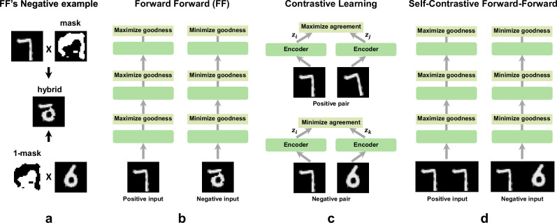
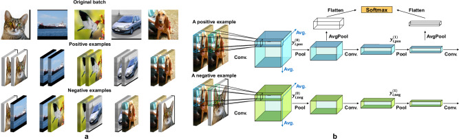
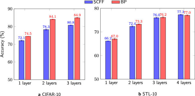
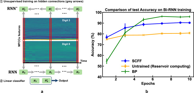
Agents that operate autonomously benefit from lifelong learning capabilities. However, compatible training algorithms must comply with the decentralized nature of these systems which imposes constraints on both the parameters counts and the computational resources. The Forward-Forward (FF) algorithm is one of these. FF relies only on feedforward operations, the same used for inference, for optimizing layer-wise objectives. This purely forward approach eliminates the need for transpose operations required in traditional backpropagation. Despite its potential, FF has failed to reach state-of-the-art performance on most standard benchmark tasks, in part due to unreliable negative data generation methods for unsupervised learning. In this work, we propose Self-Contrastive Forward-Forward (SCFF) algorithm, a competitive training method aimed at closing this performance gap. Inspired by standard self-supervised contrastive learning for vision tasks, SCFF generates positive and negative inputs applicable across various datasets. The method demonstrates superior performance compared to existing unsupervised local learning algorithms on several benchmark datasets, including MNIST, CIFAR-10, STL-10 and Tiny ImageNet. We extend FF's application to training recurrent neural networks, expanding its utility to sequential data tasks. These findings pave the way for high-accuracy, real-time learning on resource-constrained edge devices.

Fig. 1. Comparative diagram illustrating three distinct unsupervised (self-supervised) learning paradigms.

a Generation of a negative example is implemented by hybridization of two different images in the original FF paper. b In Forward Forward (FF) Learning, the layer-wise loss function is defined so as to maximize the goodness for positive inputs (real images) and minimize the goodness for negative inputs, each of which is generated by corrupting the real image to form a fake image, as shown in (a). c In Contrastive Learning, two encoders independently process input images. The model is trained to maximize agreement between the latent representations of z_i and z_j, which are obtained from two augmented views of the same image, and to minimize agreement between the representations z_i and z_k, which are derived from different images. d Our proposed Contrastive Forward Forward Learning algorithm combines the principles of Forward Forward Learning and Contrastive Learning algorithms to maximize the goodness for concatenated similar pairs and minimize the goodness for dissimilar pairs with a layer-wise loss function.

Fig. 2. SCFF method for processing with convolutional neural network architecture.

a The original batch of images (top row) is taken from the STL-10 dataset and is used to generate positive (middle row) and negative examples (bottom row) for demonstration. b The generated positive and negative examples undergo a series of convolutional (Conv.) and pooling (AvgPool or Maxpool) operations to extract relevant features. The blue axes labeled “Avg.” indicate that the goodness-based loss is computed across the channel dimension and then averaged along the height and width dimensions. Output neurons, extracted from each hidden layer via an external average pooling layer, are flattened and concatenated before being passed to a softmax layer for final classification.

Fig. 3. Comparison of test accuracy across different network depths using SCFF and backpropagation methods.

Blue and red bars represent results obtained using SCFF and Backpropagation (BP), respectively, in (a) (CIFAR-10) and (b) (STL-10). Error bars represent the mean ± standard deviation across three runs with different random seeds.

Fig. 4. Bi-directional RNN (Bi-RNN) results on FSDD dataset.

a Training procedure of SCFF on a Bi-RNN. In the first stage, unsupervised training is performed on the hidden connections (both input-to-hidden and hidden-to-hidden transformations) using positive and negative examples. Positive examples are created by concatenating two identical MFCC feature vectors of a digit along the feature dimension, while negative examples are generated by concatenating MFCCs from two different digits (e.g., digit 3 and digit 8), as illustrated in the figure. At each time step, the features are sequentially fed into the Bi-RNN (forward RNN and backward RNN^*). The red regions indicate features at different time steps. In the second stage, a linear classifier is trained using the final hidden states from both RNNs, i.e., H_T and $H_0^{*}$ as inputs for the classification task. b Comparison of test accuracy for the linear classifier trained on Bi-RNN outputs. The yellow curve represents accuracy with untrained (random) hidden neuron connections, the blue curve shows results from training with SCFF, the green curve shows Backpropagation (BP) results. Error bars represent the mean ± standard deviation across three runs with different random seeds.

Fig. 5. Probability distributions of relative positions between positive and negative examples.

a Theoretical distributions of positive examples from two different classes (denoted as Pos data 1 and Pos data 2) with distinct means (2μ₁ = 0 and 2μ₂ = 15) and identical variance (2Σ = 4) are shown with blue and orange curves, respectively. The theoretical distribution of negative examples (denoted as Neg data) derived from the two classes using the formula (7) is depicted by the grey curve. b Continuous probability density of linear discriminant analysis (LDA) applied to the IRIS dataset, displaying contours for positive examples in green (Setosa), red (Versicolor), and blue (Virginica), and for negative examples (Neg Data) in grey.

References

-
- Nahavandi, D., Alizadehsani, R., Khosravi, A. & Acharya, U. R. Application of artificial intelligence in wearable devices: opportunities and challenges. Comput. Methods Prog. Biomed.213, 106541 (2022). - PubMed
- Cardinale, M. & Varley, M. C. Wearable training-monitoring technology: applications, challenges, and opportunities. Int. J. Sports Physiol. Perform.12, 2–55 (2017). - PubMed
- Shi, W., Cao, J., Zhang, Q., Li, Y. & Xu, L. Edge computing: vision and challenges. IEEE Internet Things J.3, 637–646 (2016).
- Khouas, A. R., Bouadjenek, M. R., Hacid, H. & Aryal, S. Training machine learning models at the edge: a survey. Preprint at https://arxiv.org/abs/2403.02619 (2024).
LinkOut - more resources
Full Text Sources
Miscellaneous