. 2025 Apr 28;28(6):112536.
doi: 10.1016/j.isci.2025.112536. eCollection 2025 Jun 20.

Harnessing the analog computing power of regulatory networks with the Regulatory Network Machine

Affiliations

Harnessing the analog computing power of regulatory networks with the Regulatory Network Machine

Alexis Pietak et al. iScience. .

Abstract

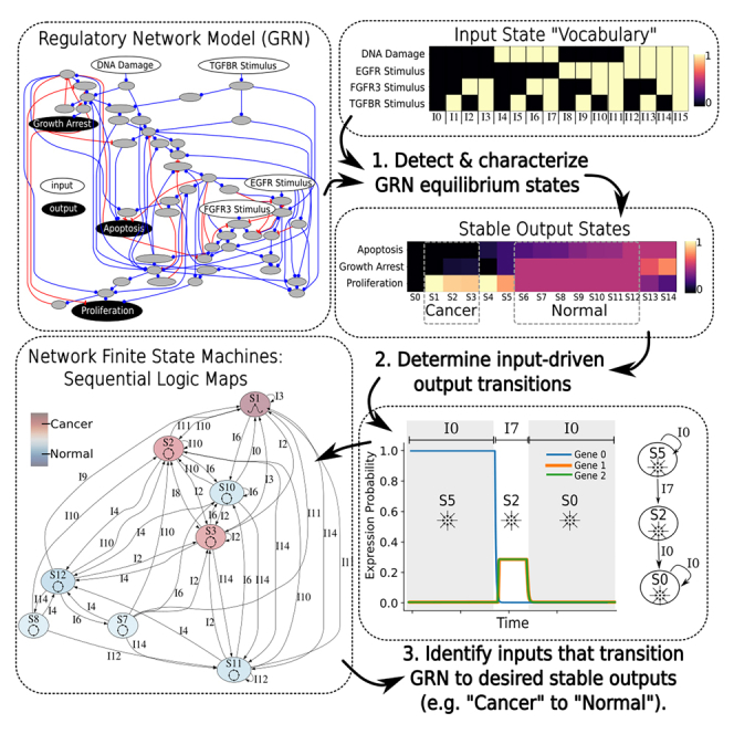
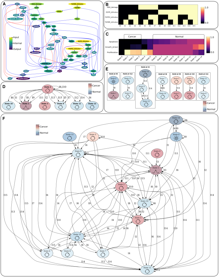
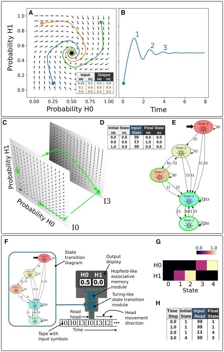
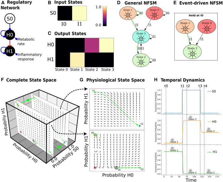
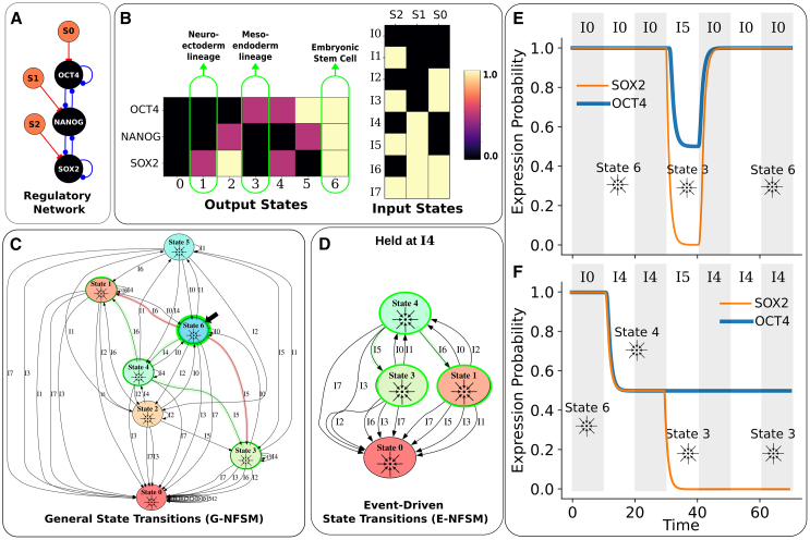
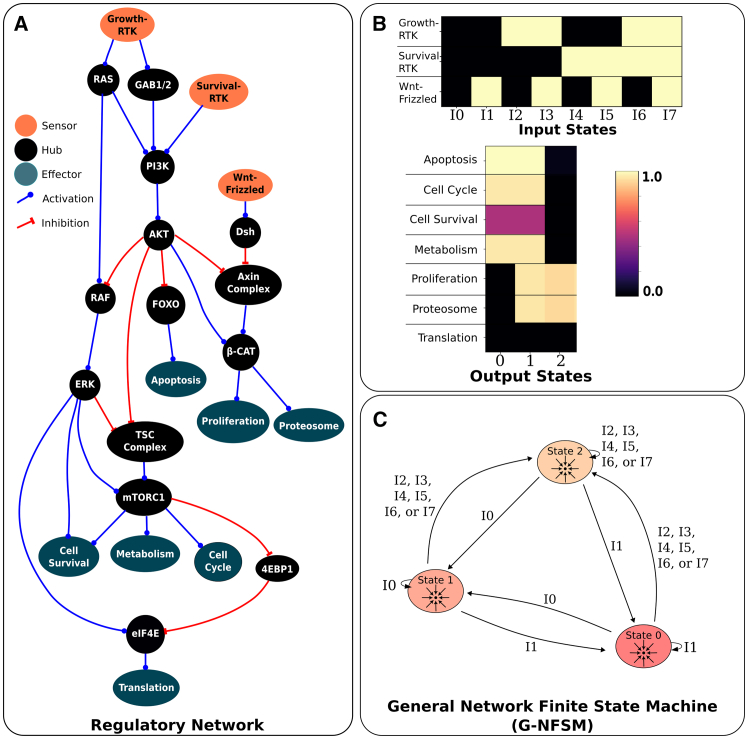
Gene regulatory networks (GRNs) are critically important for efforts in biomedicine and biotechnology. Here, we introduce the Regulatory Network Machine (RNM) framework, demonstrating how GRNs behave as analog computers capable of sophisticated information processing. Our RNM framework encapsulates: (1) a dissipative dynamic system with a focus on GRNs, (2) a set of inputs to the system, (3) system output states with identifiable relevance to biotechnological or biomedical objectives, and (4) Network Finite State Machines (NFSMs), which are maps detailing how the system changes equilibrium state in response to patterns of applied inputs. As an extension to attractor landscape analysis, the NFSMs map the sequential logic inherent in the GRN and, therefore, embody the "software-like" nature of the system, providing easy identification of specific applied interventions necessary to achieve desired, stable biological outcomes. We illustrate the use of our RNM framework in important biological examples, including in cancer renormalization.

Keywords: Bioengineering; Computer science; Systems biology.


Conflict of interest statement

M.L. is scientific co-founder and minor shareholder of Astonishing Labs, a company seeking to develop advances in regenerative medicine based on proto-cognitive properties of gene-regulatory networks. Astonishing Labs provides a sponsored research agreement to Tufts University to support this research. M.L. also has an associate faculty appointment at Harvard’s Wyss Institute. M.L. and A.P. are listed as co-inventors on a provisional patent application covering the work reported here.

Figures

None
Graphical abstract
Figure 1
Figure 1
Schematic of the persuadability spectrum In a persuadable system, simple information signals (e.g., pharmaceuticals, treats, words) can activate inherent competencies in a system to get it to emit a desired behavior, or to perform a desired function. In contrast to persuadability, a programmable system is one in which detailed information is used to precisely specify (i.e., micromanage) how a system should behave in response to different conditions and in general comes at more effort and expense than being able to persuade a system to emit desired behavior.
Figure 2
Figure 2
Complete RNM for the MAPK Cancer Cell Fate Network of Grieco et al. (A–F) The MAPK Cancer Cell Fate GRN (A) has been decomposed into: (1) an input node layer (“DNA damage”, “EGFR stimulus”, “FGFR3 stimulus”, “TGFBR stimulus”, see (B); (2) a network core (all non-input and non-output nodes in A, not shown); and (3) an output node layer (“Apoptosis”, “Growth Arrest”, and “Proliferation” nodes in (C)), representing the output responses of the network that form 15 unique equilibrium states (C). Each input node variable represents an information bit, which taken together, form 16 input “words” where the colorbar indicates expression levels (B). Each equilibrium output state is associated with an equilibrium type (e.g., point attractor, limit cycle, and to a unique expression pattern of all output nodes ((C), where colorbar indicates expression levels). Nodes in (A) are color coded to their hierarchical level. We further associate output equilibrium states with no apoptosis, low cell-cycle arrest, and high proliferation as indicative of the cancer cell state (i.e., “Apoptosis” = 0, “Growth Arrest” = 0, and “Proliferation” = 1 represents the ideal cancer state with closest state matches indicated in (B)), whereas limit cycle cell states that cycle through proliferation, cell-cycle arrest, and apoptosis expression regimes are indicative of the health cell state (B). The pathway analysis of the G-NFSM showing sustained input interventions leading from a cancer-like State 2 to healthy States 9, 10, 11, and 12 is shown in (D), where node color indicates the Euclidean distance of the equilibrium output state from the idealized cancer state. The complete set of E-NFSMs for the system are shown in (E), indicating temporary stimuli can lead to permanent transition to a cancer state (sub-graphs ‘Held at I8’ and ‘Held at I10’ in E), but that there are no temporary stimuli that can treat cancer. The full G-NFSM for the system is shown in (F), revealing all held interventions that allow for access and movement between states.
Figure 3
Figure 3
Analog computing uses dynamic systems to perform individual computations (A and B) as well as coordinated computational programs (C and D) that can be analogized to a hybrid Turing-Hopfield digital computing machine (F, G, and H) Here, dynamic systems with two time-dependent variables, ‘H0’ and ‘H1’, are considered. An analog computation is defined as a trajectory in state space, where the input is represented by initial conditions (orange, green, and blue circles in (A), the computational process is the direction-field-guided time-evolution of the system (orange, green, and blue trajectories in (A) and the output is the resulting system state (black dot in (A)). While the system in (A) functions as a homeostat, the time-evolution of the same system can be used as a counter that activates a process several times before ceasing (B). Our RNM model goes further to create a computational program using externally set inputs to a dynamic system (‘I0’ and ‘I3’ in C) to select subsets of the system’s full state space (planes in C). This has the effect of driving analog computations between equilibrium points of two state-space subsets with each change in the applied input state, creating a computational trajectory that spans the two state subspaces (green line in (C)). This allows the dynamic system to occupy multiple different equilibrium points, and to transition between these different equilibria under the influence of an applied input state, which can be organized into a state transition diagram we call the G-NFSM (E). Our RNM model can be analogized to a hybrid Turing-Hopfield digital computing machine (F, G, and H), which, like a classical Turing machine, is fed a tape of input state symbols (F) that are read by a read-head moving to the right in time (F). Yet, like a Hopfield network, the system also has associative memory, such that each state represents a pattern of output variables, which are the computational output (F and G). A detailed comparison of the properties of Turing, Hopfield, and Regulatory Network Machines is summarized in Table 2.
Figure 4
Figure 4
Here, we elucidate the core characteristics of monostable RNM computational programs using a simple 3-node regulatory network (A) with a visualizable complete state space (E) (A–G) The regulatory network studied is shown in panel (A), with input states of the system shown in (B), and the two output states in (C). The G-NFSM for the system is shown in (D). As the full state space of this system can be visualized, we can see how the transitions of the G-NFSM arise in response to applied inputs (E and F). The complete state space of the dynamic system has dimensions made of the probability of H0 expression, the probability of H1 expression, and the probability of the input S0 (E). Setting S0 = 0.0 or S0 = 1.0 selects two regions of the complete state space (two state subspaces), which each have a slice of the full direction field (E and F). The output states, State 0 and State 1 can be seen as individual equilibrium points on each state subspace plane (labeled circles ‘0’ and ‘1’ in E and F). At time t = 0.0, the system starts in an initial condition equivalent to state 0 (‘t0’ in E, F, and G) with input S0 = 0.0 applied and held (equivalent to stating that input state I0 is applied and held); in this configuration the system is in a stable equilibrium and will not change in time (G). At time t1 = 60, the input state is changed to I1 (equivalent to changing S0 = 1.0), which injects the system into the second state subspace (see E), where it is no longer in equilibrium (see t1 of E and F). The system follows the direction field of the new state subspace plane to a new equilibrium (see t2 of E, F, and G). As there is only one equilibrium state in each state subspace plane, the system output state is reversible to the original condition when the input state is changed back to I0 (see t3 and t4 of E, F, and G).
Figure 5
Figure 5
Here, we elucidate the core characteristics of multistable RNM using a simple 3-node regulatory network (A) with a visualizable complete state space (E) (A–H) The regulatory network is shown in (A), the two input states in (B), and the four output states in (C). The G-NFSM is shown in (D). We found that in some cases this system responds to transient application of input states with permanent changes to output state and therefore also has an E-NFSM (E). As the full state space of this system can be visualized, we can see how the transitions of the G-NFSM and E-NFSM arise in response to a sequence of applied inputs (F and G). The complete state space of the dynamic system has dimensions made of the probability of H0 expression, the probability of H1 expression, and the probability of the input S0 (E). Setting S0 = 0.0 or S0 = 1.0 selects two regions of the complete state space (two state subspaces), where each plane contains a functional slice of the full direction field (F and G). The multiple output states are individual equilibrium points on each state subspace plane (labeled circles ‘0’, ‘1’, ‘2’ and ‘3’ in E and F). Note that plane selected by S0 = 0.0 (input state I0) contains three unique equilibrium points and is therefore a multistable state subspace. At time t = 0.0, the system starts in an initial condition equivalent to State 1 (‘t0’ in F, G, and H) with input S0 = 0.0 (I0) applied and held; in this configuration the system is in a stable equilibrium and will not change in time (H). At time t1 = 60, the input state is changed to I1 (equivalent to changing S0 = 1.0), which injects the system into the second state subspace (see F), where it is no longer in equilibrium (see t1 of F and G). The system follows the direction field of the new state subspace plane to a new equilibrium, which corresponds to State 3 (see t2 of F, G, and H). At t3 S0 = 1.0 (input I0) is reapplied and the system is re-injected into the original state subspace, however, the system output tracks to a new output State 2 due to its new location in the state subspace and the presence of multiple equilibria altering the direction fields (see t3 and t4 of F, G, and H).
Figure 6
Figure 6
NFSM predict the emission of categorically different behaviors associated with certain input states, creating a map of both levels and modes of system behavior (A–D) Here, a cyclic regulatory network (A) with five unique output states in association with eight input states (B) forms a monostable NFSM with a limit cycle attractor as output State 1 (where all other states have point attractors) (C). Examining its behavior over time, starting the system in State 0 and holding with input state I0, then changing to input state I4, leads to a transition from a monotonically stable pattern of gene expression to a genetic oscillator, while input state I4 is applied and held (D). The genetic oscillation ceases when the input state is reverted to I0 (D). The behavior of the system is predicted by the G-NFSM, which shows the point attractor of the start state, State 0 (indicated by a black arrow and bold green halo in (C) predicted to transition to the limit cycle of State 1 (indicated by thin green halo in (C) via a transition induced by I4, and to proceed back from State 1 to State 0 via a transition induced by input I0 (C). The transitions are shown highlighted in light green (C).
Figure 7
Figure 7
Stem cell differentiation in response to transient exposure to morphogens is a context-dependent, event-driven state transition in a multistable RNM system (A–F) The ESC regulatory network modeled in this example is shown in (A). High levels of NANOG, OCT4, and SOX2 are known to correspond with undifferentiated ESC (corresponding to output State 6, (B), whereas differentiation toward a neuroectoderm lineage occurs when levels of NANOG and OCT4 drop, leaving SOX2 high (corresponding to output State 1, panel B), and differentiation toward a mesoendoderm lineage occurs when levels of NANOG and SOX2 drop, leaving OCT4 high (corresponding to output State 3, (B)). Our RNM analysis of the ESC network in (A) indicates it is a multistable system with seven unique output states (B), both a G-NFSM (C) and an E-NFSM (D), and a high average Intelligence Potential of 1.64 (see “Full Chain” network of Table 1). The biological observation of high NANOG, OCT4, and SOX2 in undifferentiated ESC indicates that the biological system starts in State 6 (marked with a black block arrow and bold green highlight in (C). The G-NFSM suggests that both States 1 and 3 are accessible from State 6 via application of input I6 and I5, respectively (trajectories highlighted in pink in (C). However, State 6 exists in monostable context I0; therefore, while transient application of I6 or I5 leads to transition of the system to State 1 or State 3, it is not a permanent change, and the system reverts to State 6 once input I6 or I5 are removed (E). The E-NFSM shows us that it is only in context I4 that a permanent change of the system from State 6 to States 1 or 3 can be achieved from a transient application of the same I6 or I5 inputs, with respective paths highlighted in green (C and D). In the time evolution of the system shown in F, we see that by first switching to State 4 with the application of I4, a transient exposure to I5 now leads to a permanent switch of the system to State 3 even with a return to the original held context established by I4 (F).
Figure 8
Figure 8
Multiple, apparently identical, systems can show dramatically different responses to the same intervention yet are deterministically described within the RNM framework (A–H) The regulatory network modeled in this example is shown in (A), which was found to have 7 unique output states (B) and to have a G-NFSM (C) and multiple E-NFSM (D). The G-NFSM shows four transitions from State 5 to four unique states (State 0, State2, State 4, and State 6) happening with the application of the same input state I7 (bold arrows of C). The E-NFSMs show four different input contexts (for systems with a baseline-normal held input state of I0, I1, I4, and I5) where State 5 transitions to another state under input I7 (bold arrows of (D)). In time-course studies, we find that systems with a held input state of I5 (E), I0 (F), I4 (G) and I1 (H) are initially stable in State 5, as predicted by the G-NFSM and E-NFSMs. Subsequent transient application of input I7 to each of the four systems leads to four different final states (E, F, G, and H), as predicted by the E-NFSMs (D).
Figure 9
Figure 9
Osmoadaptive set-point control is an analog computational system naturally “computing” the correct response required to maintain cell volume (volcell) at a target value for a wide range of environmental conditions (A–H) Here, the same physical process of osmotic-pressure-induced cell volume change is compared in an inanimate vesicle (A) and in an osmoadapted yeast cell (B). The dimensions of the systems’ full state spaces are the internal cell osmolytes (ni), cell volume (volcell), and environmental osmolyte concentrations (mo) (C–H). In the yeast cell, the osmotic process interacts with a regulatory network involving a sensor for cell volume via membrane strain (PhoQ), which conveys information regarding cell volume through to the HOG-MAPK signaling pathway, thereby altering levels of intracellular glycerol, which contributes to, and therefore allows the cell to change, total internal cell osmolytes (B). For each initial system state (an example initial state is given by the small green dot in (F) and (H)) the system dynamics naturally “compute” a new state (large green dot in (F) and (H)) by simply evolving in time under the system dynamics (green trajectory of (F) and (H)). The direction field of the inanimate vesicle maintains a surface of equilibrium states (shown as the dotted black line in (E) and (F), meaning there is a range of possible equilibrium state vesicle volumes for different environmental osmolyte concentrations and starting system states. In contrast, the yeast system’s direction field is in the form of an attractive limit cycle with a single equilibrium state appearing as a central point corresponding to the system’s desired target volume ((G) and (H), where equilibrium state/target volume are indicated by the large green dot). In 3D, the direction field for the yeast system is cylindrically-shaped, meaning the attractive limit cycle will converge to the consistent target cell volume for a wide range of environmental and internal osmolyte concentrations, thereby demonstrating that the system has excellent control of cell volume (B).
Figure 10
Figure 10
The G-NFSM is useful as a detailed set of instructions specifying which inputs engage the specific output states of signaling networks important in disease processes, such as the cross-regulation network between PAM, RAS/ERK, and Wnt/β-catenin (adapted from Figure 7 of Glaviano et al.74) (A–C) The regulatory network in A specifies activation/inhibition interactions between biologically relevant input, hub, and effector nodes, making it a suitable candidate for our RNM framework. A set of input states were defined from the input nodes (B), and three unique output states were returned from our analysis, which are shown with respect to effector node levels in B. Our analysis also determined that the dynamic system for this regulatory network is monostable, with a 1:1 reversible mapping between each input and output state, leading to a fully connected G-NFSM (C), no E-NFSM on account of its monostability, and a low Intelligence Potential of 0.8 (see ‘AKT Net’ in Table 1). The G-NFSM specifies the exact input states (as labels on transition arrows) that will result in the desired output state (C), which are intrinsic to the system and can be accessed without having to alter the network topology.

Similar articles

References

    1. Lyon P. The biogenic approach to cognition. Cogn. Process. 2006;7:11–29. - PubMed
    1. Lyon P. The cognitive cell: bacterial behavior reconsidered. Front. Microbiol. 2015;6:264. - PMC - PubMed
    1. Baluška F., Levin M. On Having No Head: Cognition throughout Biological Systems. Cogn Sci. 2016;7:902. - PMC - PubMed
    1. Gershman S.J., Balbi P.E., Gallistel C.R., Gunawardena J. Reconsidering the evidence for learning in single cells. Elife. 2021;10 - PMC - PubMed
    1. Katz Y., Springer M., Fontana W. Embodying probabilistic inference in biochemical circuits [Internet] arXiv. 2018 http://arxiv.org/abs/1806.10161 Preprint at.

LinkOut - more resources