CalTrig: A GUI-Based Machine Learning Approach for Decoding Neuronal Calcium Transients in Freely Moving Rodents

Abstract

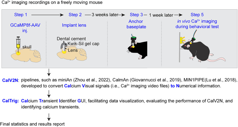
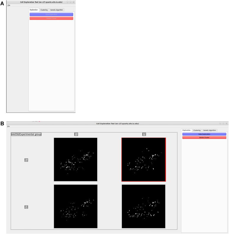
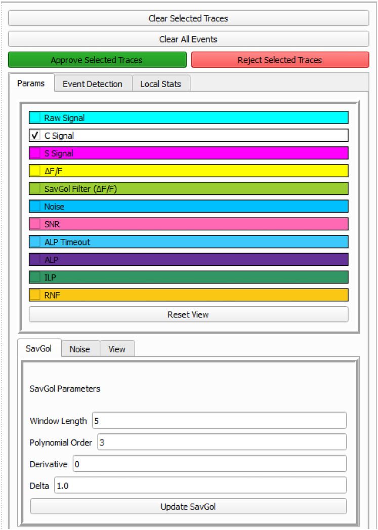
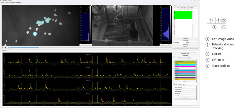
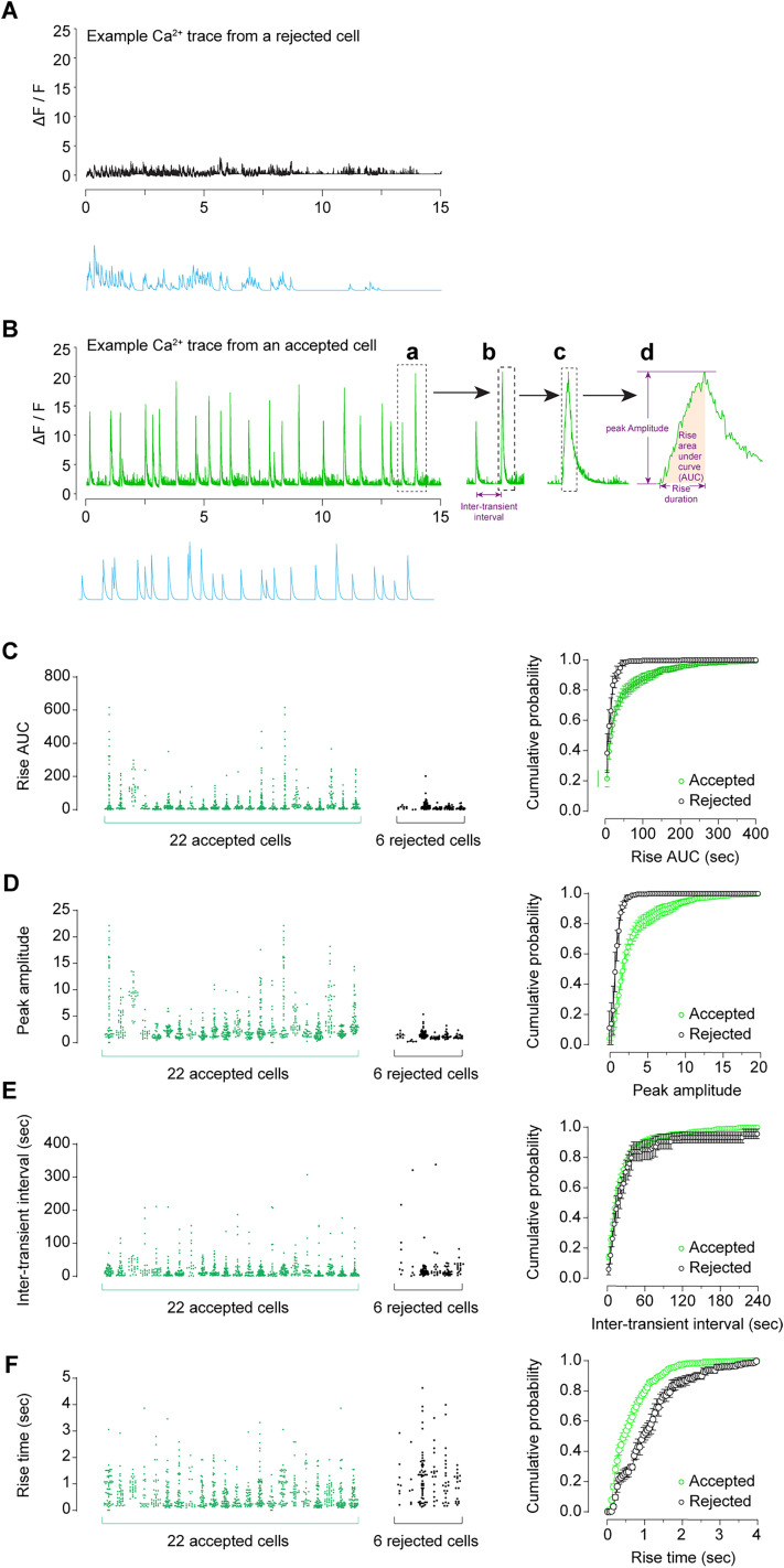
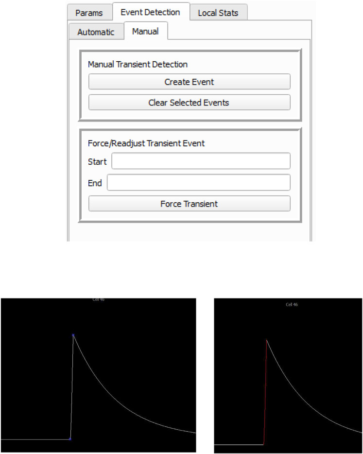
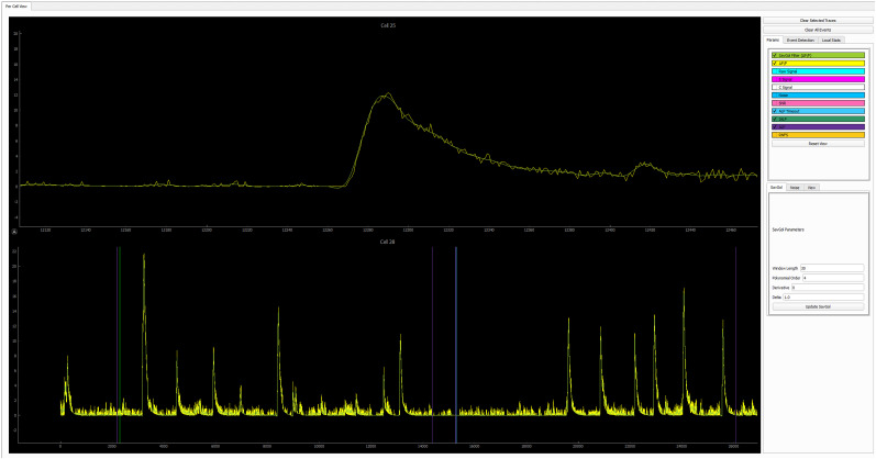
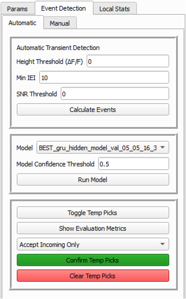
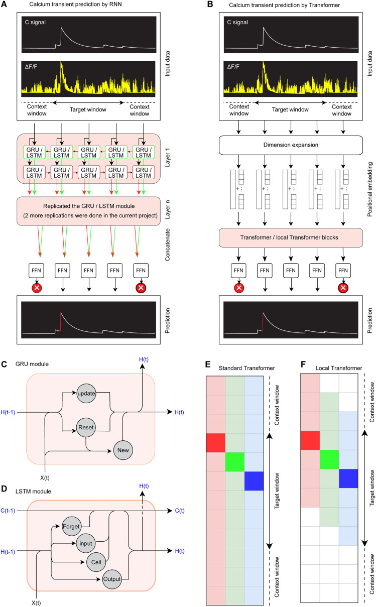
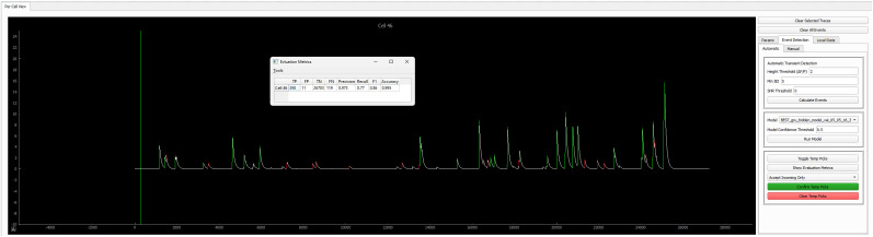
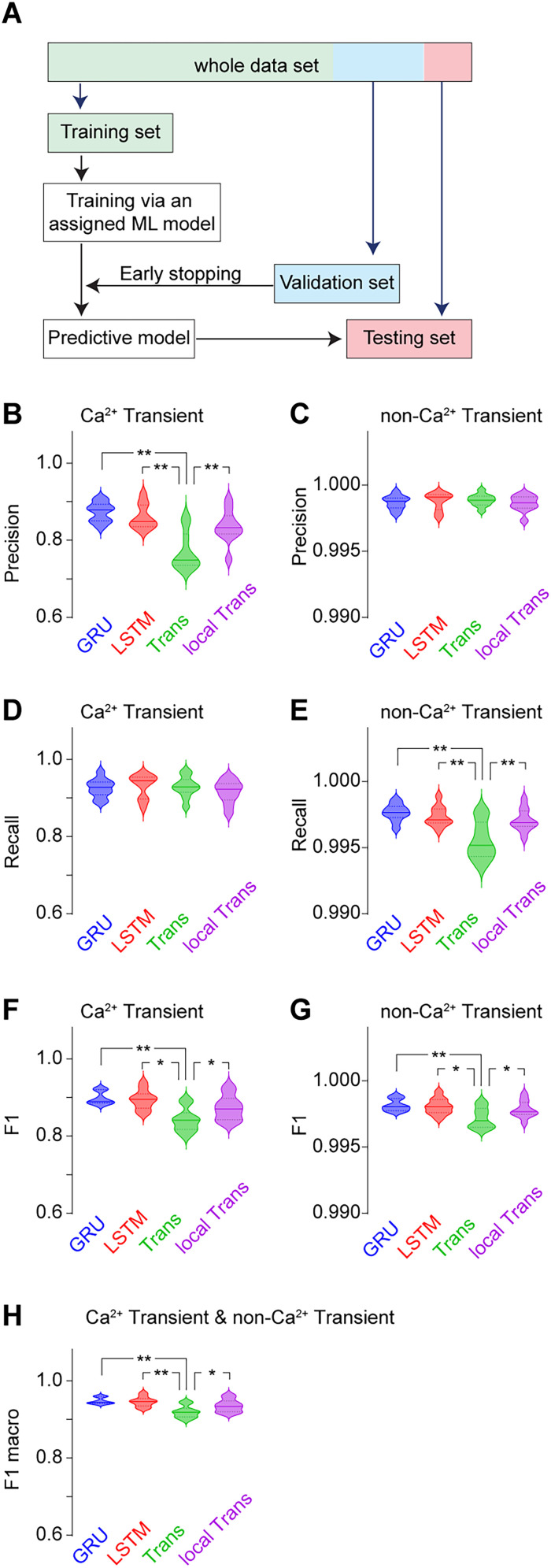
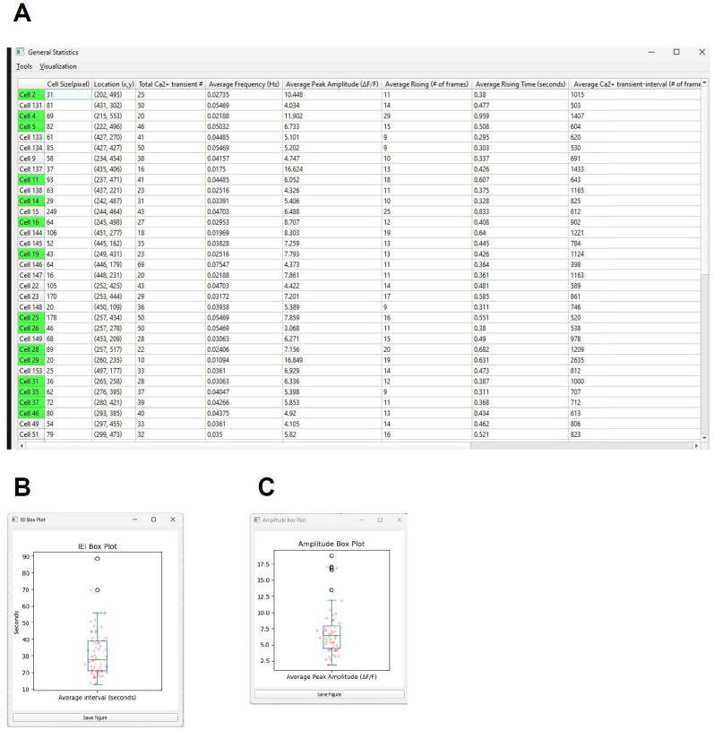
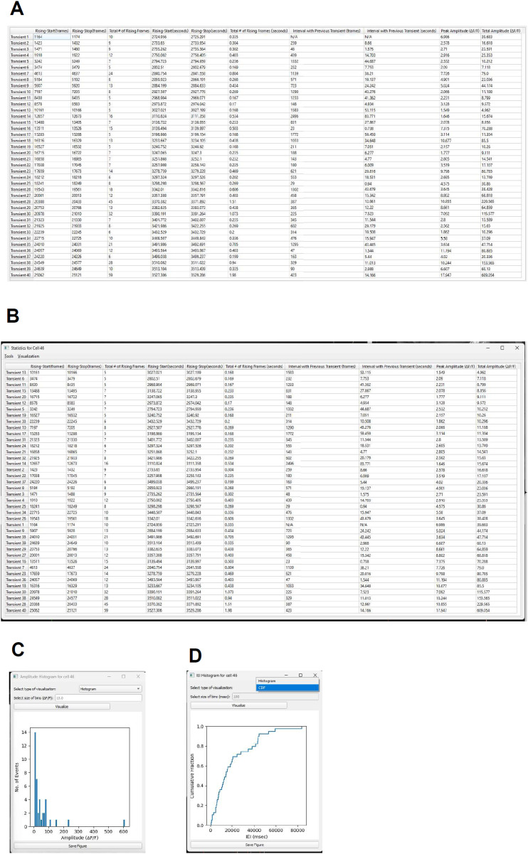
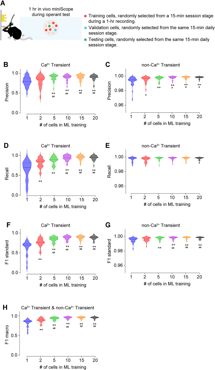
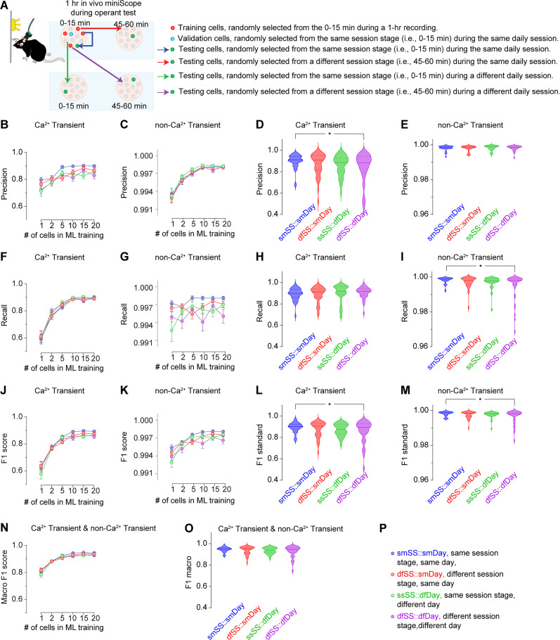
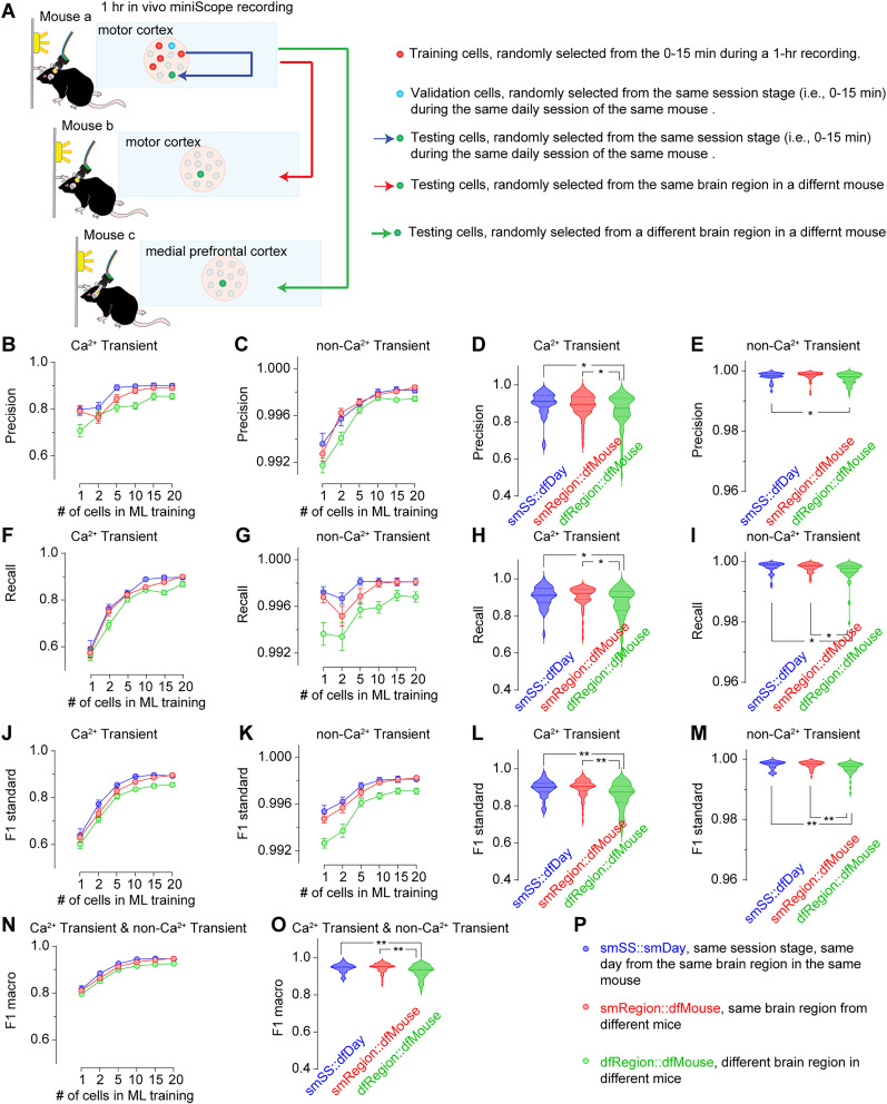
Advances in in vivo Ca²⁺ imaging using miniature microscopes have enabled researchers to study single-neuron activity in freely moving animals. Tools such as Minian and CalmAn have been developed to convert Ca²⁺ visual signals to numerical data, collectively referred to as CalV2N. However, substantial challenges remain in analyzing the large datasets generated by CalV2N, particularly in integrating data streams, evaluating CalV2N output quality, and reliably and efficiently identifying Ca²⁺ transients. In this study, we introduce CalTrig, an open-source graphical user interface (GUI) tool designed to address these challenges at the post-CalV2N stage of data processing collected from C57BL/6J mice. CalTrig integrates multiple data streams, including Ca²⁺ imaging, neuronal footprints, Ca²⁺ traces, and behavioral tracking, and offers capabilities for evaluating the quality of CalV2N outputs. It enables synchronized visualization and efficient Ca²⁺ transient identification. We evaluated four machine learning models (i.e., GRU, LSTM, Transformer, and Local Transformer) for Ca²⁺ transient detection. Our results indicate that the GRU model offers the highest predictability and computational efficiency, achieving stable performance across training sessions, different animals, and even among different brain regions. The integration of manual, parameter-based, and machine learning-based detection methods in CalTrig provides flexibility and accuracy for various research applications. The user-friendly interface and low computing demands of CalTrig make it accessible to neuroscientists without programming expertise. We further conclude that CalTrig enables deeper exploration of brain function, supports hypothesis generation about neuronal mechanisms, and opens new avenues for understanding neurological disorders and developing treatments.

Keywords: GRU; calcium transients; data visualization; in vivo calcium imaging; machine learning; miniScope.

Figure 1.

Flowchart showing the procedures of an in vivo Ca²⁺ study and highlighting the role of CalTrig in addressing gaps in data processing and analysis.

Figure 2.

Data loading. A, The front page of CalTrig serves as a hub for loading data. B, Each set of data can be visualized in the window by their cell footprint and are arranged in a grid related to the experiment design details, such as animal ID, day, and session stage.

Figure 3.

Parameter list. In top panel of the Trace Toolbox, raw signal, C signal, S signal, ΔF/F, Noise, Signal to noise ratio (SNR), as well as other behavioral readouts (e.g., active lever press, ALP; ALP during timeout; inactive lever press; and reinforcement, RNF) are listed as items to be selected to show in the Ca²⁺ trace window. The parameters of Savitzky–Golay filter (SavGol), used to estimate the SNR, are listed in the bottom panel.

Figure 4.

Five windows in CalTrig interface.

Figure 5.

Use CalTrig to validate and filter cells identified by CalV2N. This flowchart illustrates the workflow for validating and filtering cells detected by CalV2N using CalTrig. The process begins with in vivo calcium imaging data collection, followed by CalV2N analysis, which performs cell identification and calcium transient extraction. To assess the quality of detected cells, a visual exploration tool is used, allowing interactive inspection of calcium video, footprint visualization, behavioral video, and temporal traces, including raw signal, C, S, ΔF/F, noise, and signal-to-noise ratio. Users determine whether to accept or reject a detected cell based on visual confirmation of its footprint, calcium image, and calcium transients. If a cell is accepted, it proceeds to further processing for transient event confirmation. If rejected, the reasons for rejection are evaluated, which may include poor signal quality, suspicious footprint, or statistical outliers. The rejection process also considers whether the issue stems from suboptimal CalV2N performance, in which case parameters for calcium transient extraction can be optimized. If CalV2N errors persist, improvements in raw imaging data quality should be considered. See more details in Materials and Methods, Cell verification and CalV2N evaluation.

Figure 6.

Cell verification. CalTrig allows user to inspect individual cells detected by CalV2N by interactive exploration of the Ca²⁺ imaging window and Ca²⁺ trace window. A cell becomes verified after a visual confirmation of its footprint, Ca²⁺ image, and Ca²⁺ trace, ensuring identifiable Ca²⁺ transients are present. The verified cells are highlighted in green.

Figure 7.

Use CalTrig to identify Ca²⁺ transients through an integrative strategy that combines manual detection, parameter-based autodetection, and machine learning-based detection. Circled numbers (1–4) mark the corresponding steps for the four applications discussed in the main text.

Figure 8.

Add missing cell. While reviewing the Ca²⁺ imaging video, one may notice a potentially missed cell by CalV2N. CalTrig allows user to manually draw the contour of the suspected cell in the Ca²⁺ imaging window, creating its footprint. The corresponding temporal trace of signal intensity for the selected area is then calculated by averaging pixel intensities and displayed in the Ca²⁺ trace window. If the Ca²⁺ traces meet the criteria for accepted cells, the manually identified cell can be added to the list of missing cells.

Figure 9.

Ca²⁺ transient dynamics in accepted and rejected cells. A, Example Ca²⁺ transient traces from a rejected cell. B, Example Ca²⁺ transient traces from an accepted cell. a → b, the dash-framed trace in a was horizontally enlarged to illustrate the measurement of ITI. b → c, the dash-framed trace in b was further horizontally enlarged to illustrate the rise and decay of a Ca²⁺ transient. c → d, the dash-framed trace in c was further horizontally enlarged to illustrate the measurements of peak amplitude, the rise AUC, and the rise time. C, The individual rise AUC values of Ca²⁺ transients from 22 accepted cells and 6 rejected cells in M2 randomly selected from a mouse, and the summary data showing the different cumulative probability between accepted versus rejected cells, indicating that accepted cells exhibit more Ca²⁺ transients with larger rise AUC values compared with rejected cells. D, The individual peak amplitude values of Ca²⁺ transients from 22 accepted cells and 6 rejected cells in M2 randomly selected from a mouse, and the summary data showing the different cumulative probability between accepted versus rejected cells, indicating that accepted cells exhibit more Ca²⁺ transients with larger peak amplitude values compared with rejected cells. E, The individual ITI values of Ca²⁺ transients from 22 accepted cells and 6 rejected cells in M2 randomly selected from a mouse, and the summary data showing the similar cumulative probability between accepted versus rejected cells. F, The individual rise time values of Ca²⁺ transients from 22 accepted cells and 6 rejected cells in M2 randomly selected from a mouse, and the summary data showing the different cumulative probability between accepted versus rejected cells, indicating that accepted cells exhibit less Ca²⁺ transients with larger long rise time compared with rejected cells.

Figure 10.

Manual identification of Ca²⁺ transients. Ca²⁺ transients can be directly identified by manually selecting the start and end points of the rising section of Ca²⁺ transients.

Figure 11.

Savitzky–Golay filter. This sets the minimal signal-to-noise ratio (SNR). Using the Savitzky–Golay filter (Steinier et al., 1972; Dai et al., 2017) to smooth ΔF/F signals, noise is calculated as the difference between the original and filtered ΔF/F, further smoothed by a rolling window strategy. Then SNR is computed by dividing the smoothed ΔF/F by the estimated noise.

Figure 12.

Automatic detection. To enhance detection accuracy, the parameter-based autodetection algorithm starts by including all C peaks in a candidate pool and then filtering down to a valid subset based on three predefined parameters: “Peak Threshold (ΔF/F),” “Interval Threshold,” and “SNR Threshold.”

Figure 13.

Flowchart demonstrating Ca²⁺ transient validation via machine learning models. A, Application of RNNs in predicting Ca²⁺ transients. The input consists of the C signal and ΔF/F traces. A sequence of GRUs or LSTM modules processes the temporal dynamics of the Ca²⁺ transient. The network includes multiple stacked layers, with fully connected layers (FNN) at the final stage to produce the predicted Ca²⁺ transient. B, Application of Transformer models for predicting Ca²⁺ transients. The input is first expanded through a dimensional transformation step, followed by repeated attention-based self-mapping in either a standard Transformer or a local Transformer architecture. The processed features are then passed through a feedforward network (FNN) to generate the predicted Ca²⁺ transient. C, D, Diagrams showing the internal operations of two variants of RNN, i.e., GRU module (C) and LST module (D). The GRU uses two gates: the update gate, which controls the amount of information passed to the next step, and the reset gate, which determines how much of the previous information to forget. These gates modify the hidden state H(t) at the current time-step based on the input X(t) and the previous hidden state H(t−1), leading to a new hidden state H(t). The LSTM module architecture is depicted, showcasing its cell structure. It uses three gates: forget, input, and output gates to control the flow of information. The input X(t), the previous cell state C(t−1), and the previous hidden state H(t−1) are processed through these gates to update the cell state C(t) and produce the new hidden state H(t). E, F, Diagram showing the Transform (E) and local Transformer (F) mechanisms. Multiple columns represent the same set of data. Nontranslucent colored regions highlight the specific values being processed, while translucent colors represent comparison values within the self-attention mechanism. No color denotes values excluded from evaluation, enforcing global attention to all time points. Local Transformer mechanism. Unlike the standard Transformer, the local Transformer focuses only on a subset of adjacent time points, restricting the attention scope to a local temporal window. This reduces computational complexity while maintaining essential local dependencies in Ca²⁺ transient predictions. Data input format: The models receive sequential time-series data of C signals and ΔF/F traces as input. Data output format: The models predict Ca²⁺ transients by generating the time stamp of the initial and ending frame for each Ca²⁺ transients, which will be saved in E. FNN, Feedforward neural network.

Figure 14.

Machine learning evaluation. We used Precision, Recall, F1, and macro F1 as key metrics to evaluate the performance of machine learning model in predicting Ca²⁺ transients versus non-Ca²⁺ transients.

Figure 15.

GRU module has the best predictability of Ca²⁺ transients. A, Shared strategy for assigning data to training, validation, and testing across four machine learning models. B, C, Precision varied significantly in Ca²⁺ transient prediction (B, F_(3,36) = 14.2, p < 0.01), but remained similar in no Ca²⁺ transient prediction (C, F_(3,36) = 0.4, p = 0.78) in four machine learning models. D, E, Recall remained similar in Ca²⁺ transient prediction (D, F_(3,36) = 0.6, p = 0.63) but varied in Ca²⁺ transient prediction (E, F_(3,36) = 9.4, p < 0.01) in four machine learning models. F,G, Significant differences in F1 scores of Ca²⁺ transient prediction (F, F_(3,36) = 9.3, p < 0.01) and no Ca²⁺ transient prediction (G, F_(3,36) = 4.8, p < 0.01) in four machine learning models. H, Significant differences in macro F1 scores (F_(3,36) = 9.3, p < 0.01) in four machine learning models. Each machine learning model was trained using data from 226 cells from 4 mice, with 28 cells allocated to the validation set and 28 cells to the testing set. Each experimental group consisted of 10 tests. Data were analyzed by one-way ANOVA, followed by Bonferroni post hoc test. *p < 0.05; **p < 0.01.

Figure 16.

Animal-wide data export. A, A data table is generated, with each row representing one of the CalS2N-detected cells and each column providing specific readout as a general description of that cell. B, C, Average peak amplitude (B) and inter-transient interval (ITI, C) can be directly generated and saved as edit able SVG files for publication purposes.

Figure 17.

Cell-wide data export. A, A data table is generated for a selected cell, with the top row displaying column titles and the subsequent rows representing individual Ca²⁺ transients detected by CalTrig, one transient per row. B, The column title (e.g., Total Amplitude) can be selected to sort the data based on the information in the selected column. C, D, Figures such as amplitude distribution (C) and ITI frequency histograms (D) can be created directly from this data and saved as editable SVG files for publication.

Figure 18.

Prediction of Ca²⁺ transients or no Ca²⁺ transients across different numbers of cells in machine learning training. A, Strategy of randomly picking up cells for training, validation, and testing within the same session stage on the same day. B,C, Increasing the number of cells in machine learning training model significantly improved the precision in predicting Ca²⁺ transients (B, F_(5,234) = 11.0, p < 0.01) and no Ca²⁺ transients (C, F_(5,234) = 12.8, p < 0.01). D, E, Increasing the number of cells in machine learning training model significantly improved the recall in predicting Ca²⁺ transients (D, F_(5,234) = 40.9, p < 0.01) and no Ca²⁺ transients (E, F_(5,234) = 2.8, p = 0.02). F,G, Increasing the number of cells in machine learning training model significantly improved the F1 scores in predicting Ca²⁺ transients (F, F_(5,234) = 46.7, p < 0.01) and no Ca²⁺ transients (G, F_(5,234) = 12.0, p < 0.01). H, Increasing the number of cells in machine learning training model significantly improved the macro F1 scores in predicting Ca²⁺ transients and no Ca²⁺ transients (H, F_(5,234) = 46.6, p < 0.01). Data were obtained using the GRU model. Each experimental group consisted of 10 tests per mouse, with 4 mice per group, resulting in a total of 40 data points per experimental group. Data were analyzed by one-way ANOVA, followed by Bonferroni post hoc test. *p < 0.05; **p < 0.01, compared with the machine learning model trained by 1 cell. ^#p < 0.05; ^##0.01, compared with the machine learning model trained by 2 cells. 40 testing cells in each group.

Figure 19.

Prediction of Ca²⁺ transients or no Ca²⁺ transients within the same mice. A, Four strategies for sourcing cells within the M2 area from a mouse for machine learning model training, validation, and testing. B–E, The training cell number, and the testing cell source, but not their interactions, significantly affected the Precision in predicting Ca²⁺ transients (B, training cell # F_(5,936) = 21.4, p < 0.01; testing cell source F_(3,936) = 10.0, p < 0.01; training cell number × testing cell source interaction F_(15,936) = 0.8, p = 0.64). The training cell number, but not the testing cell source or their interactions, affected the Precision in predicting no Ca²⁺ transients (C, training cell number F_(5,936) = 71.7, p < 0.01; testing cell source F_(3,936) = 1.1, p = 0.36; training cell number × testing cell source interaction F_(15,936) = 0.3, p = 0.99). When 20 cells were included in the machine learning training model, the Precision in predicting Ca²⁺ transients (D, F_(3,156) = 2.7, p = 0.046), but not in predicting no Ca²⁺ transients (E, F_(3,156) = 0.2, p = 0.93), in testing cells from different session stage on different day reduced. F–I, The training cell number, but not the testing cell source or their interactions, significantly affected the Recall in predicting Ca²⁺ transients (F, training cell number F_(5,936) = 126.0, p < 0.01; testing cell source F_(3,936) = 0.8, p = 0.49; training cell number × testing cell source interaction F_(15,936) = 0.3, p = 0.99). The number of cells, the testing cell source, but not their interactions, significantly affected the Recall in predicting no Ca²⁺ transients (G, training cell number F_(5,936) = 2.7, p = 0.02; testing cell source F_(3,936) = 11.4, p < 0.01; training cell number × testing cell source interaction F_(15,936) = 1.5, p = 0.10). When 20 cells were included in the machine learning training model, the Recall in predicting no Ca²⁺ transients (I, F_(3,156) = 3.3, p = 0.02), but not in predicting the Ca²⁺ transients (H, F_(3,156) = 0.4, p = 0.78), in testing cells from different session stage on different day reduced. J–M, The training cell number and the testing cell source, but not their interactions, significantly affected the F1 scores in predicting Ca²⁺ transients (J, training cell number F_(5,936) = 130.0, p < 0.01; testing cell source F_(3,936) = 3.0, p = 0.03; training cell number × testing cell source interaction F_(15,936) = 0.7, p = 0.74). Similarly, the number of cells and the testing cell source, but not their interactions, significantly affected the F1 scores in predicting no Ca²⁺ transients (K, training cell number F_(5,936) = 32.3, p < 0.01; testing cell source F_(3,936) = 8.8, p < 0.01; training cell number × testing cell source interaction F_(15,936) = 1.2, p = 0.28). When 20 cells were included in the machine learning training model, the Recall in predicting Ca²⁺ transients (L, F_(3,156) = 2.7, p = 0.048) and no Ca²⁺ transients (M, F_(3,156) = 2.8, p = 0.040) in testing cells from different session stage on different day reduced. N, O, The training cell number, and the testing cell source, but not their interactions, significantly affected the macro F1 scores in predicting Ca²⁺ transients and no Ca²⁺ transients (N, training cell number F_(5,936) = 128.5, p < 0.01; testing cell source F_(3,936) = 3.1, p = 0.03; training cell number × testing cell source interaction F_(15,936) = 0.8, p = 0.73). When 20 cells were included in the machine learning training model, the macro F1 scores in predicting Ca²⁺ transients and no Ca²⁺ transients (O, F_(3,156) = 2.8, p = 0.041) in testing cells from different session stage on different day reduced. P, Legends showing the color-coded abbreviations for four experimental groups. Data were obtained using the GRU model. Each experimental group consisted of 10 tests per mouse, with 4 mice per group, resulting in a total of 40 data points per experimental group. Data were analyzed by two-way ANOVA (B,C,F,G,J,K,N) or one-way ANOVA (D,E,H,I,L,M,O), followed by Bonferroni post hoc test. *p < 0.05; **p < 0.01. 40 testing cells in each group.

Figure 20.

Prediction of Ca²⁺ transients or no Ca²⁺ transients in different mice. A, Three strategies for sourcing testing cells (smSS::smDay, between mice, different regions, see more details in panel P). B–E, The training cell number, and the testing cell source, but not their interactions, significantly affected the Precision in predicting Ca²⁺ transients (B, training cell number F_(5,942) = 24.4, p < 0.01; testing cell source F_(2,942) = 19.2, p < 0.01; training cell number × testing cell source interaction F_(10,942) = 1.1, p = 0.37) and the no Ca²⁺ transients (C, training cell number F_(5,942) = 74.1, p < 0.01; testing cell source F_(2,942) = 11.6, p < 0.01; training cell number × testing cell source interaction F_(10,942) = 1.0, p = 0.43). When 20 cells were included in the machine learning training model, the Precision in predicting Ca²⁺ transients (D, F_(2,157) = 4.7, p = 0.01) and no Ca²⁺ transients (E, F_(2,157) = 6.2, p < 0.001) in testing cells from different regions in different mice reduced. F–I, The training cell number, but not the testing cell source or their interactions, significantly affected the Recall in predicting Ca²⁺ transients (F, training cell number F_(5,942) = 145.6, p < 0.01; testing cell source F_(2,942) = 3.7, p = 0.02; training cell number × testing cell source interaction F_(10,942) = 0.7, p = 0.68). The training cell number and the testing cell source, but not their interactions, significantly affected the Recall in predicting no Ca²⁺ transients (G, training cell number F_(5,942) = 8.7, p < 0.01; testing cell source F_(2,942) = 22.9, p < 0.01; training cell number × testing cell source interaction F_(10,942) = 0.9, p = 0.58). When 20 cells were included in the machine learning training model, the Recall in predicting Ca²⁺ transients (H, F_(2,157) = 4.4, p = 0.01) and no Ca²⁺ transients (I, F_(2,157) = 5.3, p < 0.01) in testing cells from different regions in different mice reduced. J–M, The training cell number, and the testing cell source, but not their interactions, significantly affected the F1 scores in predicting Ca²⁺ transients (J, training cell number F_(5,942) = 165.7, p < 0.01; testing cell source F_(2,942) = 17.6, p < 0.01; training cell number × testing cell source interaction F_(10,942) = 0.3, p = 0.98) and the no Ca²⁺ transients (K, training cell number F_(5,942) = 55.8, p < 0.01; testing cell source F_(2,942) = 40.4, p < 0.01; training cell number × testing cell source interaction F_(10,942) = 1.3, p = 0.23). When 20 cells were included in the machine learning training model, the F1 scores in predicting Ca²⁺ transients (L, F_(2,157) = 8.9, p < 0.01) and no Ca²⁺ transients (M, F_(2,157) = 9.3, p < 0.01) in testing cells from different regions in different mice reduced. N, O, The training cell number, and the testing cell source, but not their interactions, significantly affected the macro F1 scores in predicting Ca²⁺ transients and no Ca²⁺ transients (N, training cell number F_(5,942) = 164.6, p < 0.01; testing cell source F_(2,942) = 18.3, p < 0.01; training cell number × testing cell source interaction F_(10,942) = 0.3, p = 0.98). When 20 cells were included in the machine learning training model, the macro F1 scores in predicting Ca²⁺ transients and no Ca²⁺ transients (O, F_(2,157) = 9.0, p < 0.01) in testing cells from different regions in different mice reduced. P, Legends showing the color-coded abbreviations for four experimental groups. Data were obtained using the GRU model. Each experimental group consisted of 10 tests per mouse, with 4 mice for smSS::smDay, and 6 mice for smRegion::dfMouse and dfRegion::dfMouse, resulting in a total of 40 data points for smSS::smDay and 60 data points for smRegion::dfMouse and dfRegion::dfMouse. Data were analyzed by two-way ANOVA (B,C,F,G,J,K,N) or one-way ANOVA (D,E,H,I,L,M,O), followed by Bonferroni post hoc test. *p < 0.05; **p < 0.01. 40 testing cells in each group.

References

1. Alfattni G, Peek N, Nenadic G (2021) Attention-based bidirectional long short-term memory networks for extracting temporal relationships from clinical discharge summaries. J Biomed Inform 123:103915. 10.1016/j.jbi.2021.103915 - DOI - PubMed
1. Bao Y, Soltanian-Zadeh S, Farsiu S, Gong Y (2021) Segmentation of neurons from fluorescence calcium recordings beyond real time. Nat Mach Intell 3:2. 10.1038/s42256-020-00281-z - DOI - PMC - PubMed
1. Bian Q, As’arry A, Cong X, Rezali K, Raja Ahmad R (2024) A hybrid transformer-LSTM model apply to glucose prediction. PLoS One 19:e0310084. 10.1371/journal.pone.0310084 - DOI - PMC - PubMed
1. Boffi NM, Vanden-Eijnden E (2024) Deep learning probability flows and entropy production rates in active matter. Proc Natl Acad Sci U S A 121:e2318106121. 10.1073/pnas.2318106121 - DOI - PMC - PubMed
1. Chandra A, Tunnermann L, Lofstedt T, Gratz R (2023) Transformer-based deep learning for predicting protein properties in the life sciences. eLife 12:e82819. 10.7554/eLife.82819 - DOI - PMC - PubMed
LinkOut - more resources