From pixels to planning: scale-free active inference

Abstract

This paper describes a discrete state-space model and accompanying methods for generative modeling. This model generalizes partially observed Markov decision processes to include paths as latent variables, rendering it suitable for active inference and learning in a dynamic setting. Specifically, we consider deep or hierarchical forms using the renormalization group. The ensuing renormalizing generative models (RGM) can be regarded as discrete homologs of deep convolutional neural networks or continuous state-space models in generalized coordinates of motion. By construction, these scale-invariant models can be used to learn compositionality over space and time, furnishing models of paths or orbits: that is, events of increasing temporal depth and itinerancy. This technical note illustrates the automatic discovery, learning, and deployment of RGMs using a series of applications. We start with image classification and then consider the compression and generation of movies and music. Finally, we apply the same variational principles to the learning of Atari-like games.

Keywords: Bayesian model selection; active inference; active learning; compression; network-physiology; renormalization group; structure learning.

FIGURE 1

Generative models. A generative model specifies the joint probability of observable consequences and their hidden causes. Usually, the model is expressed in terms of a likelihood (the probability of consequences given their causes) and priors (over causes). When a prior depends on a random variable, it is called an empirical prior. Here, the likelihood is specified by a tensor A, encoding the probability of an outcome under every combination of states (s). Priors over transitions among hidden states, B, depend on paths (u), whose transition probabilities are encoded in C. Certain (control) paths are more probable a priori if they minimize their expected free energy (G), expressed in terms of risk and ambiguity (white panel). If the path is not controllable, it remains fixed over the epoch in question, where E specifies the prior over paths. The left panel provides the functional form of the generative model in terms of categorical (Cat) distributions that are themselves parameterized as Dirichlet (Dir) distributions, equipping the model with the parametric depth. The lower equalities list the various operators required for variational message passing in Figure 2. These functions are taken to operate on each column of their tensor arguments. The graph on the lower left depicts the generative model as a probabilistic graphical model that foregrounds the implicit temporal depth implied by priors over state transitions and paths. This example shows dependencies for fixed paths. When equipped with hierarchical depth, the POMDP acquires a separation of temporal scales. This follows because higher states generate a sequence of lower states, that is, the initial state (via the D tensor) and subsequent path (via the E tensor). This means higher levels unfold more slowly than lower levels, furnishing empirical priors that contextualize the dynamics of their children. At each hierarchical level, hidden states and accompanying paths are factored to endow the model with factorial depth. In other words, the model “carves nature at its joints” into factors that interact to generate outcomes (or initial states and paths at lower levels). The implicit context-sensitive contingencies are parameterized by tensors mapping from one level to the next (D and E). Subscripts pertain to time, while superscripts denote distinct factors (f), outcome modalities (g), and combinations of paths over factors (h). Tensors and matrices are denoted in uppercase bold, while posterior expectations are in lowercase bold. The matrix π encodes the probability over paths under each policy (for notational simplicity, we have assumed a single control path). The ⊙ notation implies a generalized inner (i.e., dot) product or tensor contraction, while × denotes the Hadamard (element by element) product. ψ(·) is the digamma function applied to the columns of a tensor.

FIGURE 2

Belief updating and variational message passing: the right panel presents the generative model as a factor graph, where the nodes (square boxes) correspond to the factors of the generative model (labeled with the associated tensors). The edges connect factors that share dependencies on random variables. The leaves of filled circles correspond to known variables, such as observations (o). This representation is useful because it scaffolds the message passing—over the edges of the factor graph—that underwrites inference and planning. The functional forms of these messages are shown in the left-hand panels, where the panels labels (A–E) indicate the corresponding tensors in the factor graph on the right., where the panels labels (A–E) indicate the corresponding tensors in the factor graph on the right. For example, the expected path in the first equality of panel (C) is a softmax function of two messages. The first is a descending message ${\mu }_{\downarrow \mathbf{E}}^f$ from (E) that inherits from expectations about hidden states at the level above. The second is the log-likelihood of the path based on expected free energy, G. This message depends on Dirichlet counts scoring preferred outcomes—that is, prior constraints on modality g—encoded in c ^g : see Figure 1 and Equation 2. The two expressions for ${\mu }_{\mathbf{C}}^f$ correspond to fixed and control paths, respectively. The updates in the lighter panels correspond to learning, that is, updating Bayesian beliefs about parameters. Similar functional forms for the remaining messages can be derived by direct calculation. The ⊙ notation implies a generalized inner product or tensor contraction, while ⊗ denotes an outer product. ch (·) and pa (·) return the children and parents of latent variables.

FIGURE 3

Renormalizing generative model. This graphical model illustrates the architecture of renormalizing generative models (temporal renormalization has been omitted for clarity). In these models, the latent states at any given level generate the initial conditions and paths of [groups of] states at the lower level (red box). This means that the trajectory over a finite number of timesteps at the lower level is generated by a higher state. This entails a separation of temporal scales and implicit renormalization, such that higher states only change after a fixed number of lower state transitions. This kind of model can be specified in terms of (i) transition tensors (B) at each level, encoding transitions under each discrete path, and (ii) likelihood mappings between levels, corresponding to the D and E tensors of previous figures. These can be treated as subtensors of likelihood mappings ${\mathbf{A}}^n=\left\{{\mathbf{D}}_1^n,{\mathbf{E}}_1^n,{\mathbf{D}}_2^n,{\mathbf{E}}_2^n,\dots \right\}$ that furnish empirical priors over the states (and paths) at each level (n). Because each state (and path) has only one parent, the ensuing Markov blanket (blue circles) of each state (red circle) ensures conditional independence among latent factors. In summary, a renormalizing generative model (RGM) is a hypergraph, parameterized by two sorts of (A and B) tensors, in which the children of states at any level bipartition into initial states and paths. In this example, the blocking transformation groups pairs of states (and paths).

FIGURE 4

Quantizing images. The left panel shows an example of an MNIST image after resizing to 32 pixels × 32 pixels, following histogram equalization. The image in the right panel corresponds to the image in pixel space generated by quantized singular variates, used to form a linear mixture of singular vectors over groups of pixels. The centers of the (4 × 4) groups of pixels are indicated by the small red dots (encircled in white). In this example, the singular variates could take seven discrete values centered on zero for a maximum of 16 singular vectors. At subsequent levels, (2 × 2) groups of groups are combined via grouping or blocking operators. The centroids of these groups (of groups) at the three successive scales are shown with successively larger red dots. At the third scale, there are four groups corresponding to the quadrants of the original image.

FIGURE 5

Renormalizing likelihoods. This figure is a schematic representation of the composite likelihood mappings (comprising D and E) among the levels of an RGM, following fast structure learning. In each of these graphics, black indicates a nonzero element, and white indicates a zero element. In the lower row of matrices, the columns of the matrices are the alternative possible values of states at that level, concatenated for all state factors. The rows are the possible values for states (or observations) at the level below, similarly concatenated. By the third level, each latent state can generate an entire image via recursive application of sparse, block-diagonal matrices, where “nz” counts the number of nonzero elements. In this example, the model has been equipped with a fourth level, mapping from 10 digit classes to 130 latent states at the third level (encoding 13 images of 10 digits). These likelihood mappings (that mediate empirical priors) are assembled automatically during structure learning by accumulating unique combinations of (recursively grouped) states at subordinate levels. The upper row reproduces the matrices of the lower row after transposition to illustrate the dimension reduction inherent in the grouping of states. Each transposed matrix is shifted one to the left relative to the lower row. This means the states generated by the upper matrices are represented in the columns, aligning with the states in the conditioning sets in the columns of the matrices below. For example, the thousand or so states at the second level generate over 6,000 states at the first, which specify the mixture of singular vectors required to generate an image. Similarly, the 500 or so states at level 3 generate empirical priors over a partition of level 2 states into four subsets or groups (the first is highlighted in cyan), and so on. Crucially, by construction, the children of states at any level constitute a partition, such that every child is included in exactly one subset. This means that states at any level have only one parent, rendering the subsets of the partition at the higher level conditionally independent. In other words, there are no conditionally dependent co-parents. This enables efficient sum–product operations during model inversion because one must only compute dot products of subtensors (i.e., small matrices) specified by the parents of a group. Note that the matrices in this figure are not simple likelihood mappings: they are concatenated likelihood mappings from all hidden states at one level to all hidden states (and paths) at the subordinate level, where the sum to one constraint is applied to the states (or paths) each child could be in.

FIGURE 6

Renormalization and projective fields. This figure shows exemplar projective fields of the (MNIST) RGM in terms of posterior predictive densities in pixel space associated with states at successive levels (or scales) in the generative model. The top row corresponds to the posterior predictions of the first eight states at the fourth level, while subsequent rows show the differences in posterior predictions obtained by switching the first state for the subsequent eight states at each level. The key thing to note is that the sizes of the projective fields become progressively smaller and more localized as we descend scales or levels.

FIGURE 7

Active learning. This figure reports the assimilation or active learning of the training MNIST dataset. In this example, images were assimilated if, and only if, they increased the expected free energy of the RGM. In the absence of prior preferences or constraints, this ensures minimum information loss by underwriting informative likelihood mappings at each level (i.e., maximizing mutual information). The left panel reports the mutual information as a function of ingesting 10,000 training images. The left panel reports the mutual information at the first level (blue line) and intermediate levels. The middle panel reports the mutual information at the final (fourth) level. The dashed lines correspond to the maximum mutual information that could be encoded by the likelihood mappings. The right panel shows the corresponding evidence lower bound (negative variational free energy), scored by inferring the latent states (digit class) generating each image. The fluctuations here reflect the fact that some images are more easily explained than others under this model. As the model improves, there are progressively fewer images with a very low evidence lower bound (ELBO): that is, −16 natural units or fewer.

FIGURE 8

Classification and confidence. This figure reports classification performance following the learning described in Figure 7. Because inverting a generative model corresponds to inference, recognition, or classification, one can evaluate the posterior over latent causes—here, digit class—and the marginal likelihood (i.e., model evidence) of an image while accommodating uncertainty about its class. This means that one can score the probability that each image was caused by any digit class in terms of the ELBO. The distribution of the ELBO over the 10,000 training images is shown as a histogram in the left panel (for correctly classified images). The smaller histogram (foregrounded) shows the distribution of log-likelihoods for the subset of images that were classified incorrectly. Having access to the marginal likelihood means that one can express classification accuracy as a function of the (marginal) likelihood the image was generated by a digit. The ensuing classification accuracy is shown in the right panel as a function of a threshold (c.f., Occam’s window) on the ELBO or evidence that each image was generated by a digit. The vertical dashed lines show the median ELBO (−13.85 nats). Classification accuracy for all images was only 95.1%. However, the accuracy rises to 99.8% following a median split based on their marginal likelihoods.

FIGURE 9

Classification failures. This figure provides examples of incorrect classification of images with a small marginal likelihood. Each pair of images presents the training image with its label and the corresponding posterior prediction in pixel space and accompanying maximum a posteriori classification.

FIGURE 10

A dove in flight. This figure shows a frame from a movie of a (digital) dove flapping her wings. The left panel is a TrueColor (128 pixels × 128 pixels, RGB) image used for structure learning, while the right panel shows the corresponding posterior prediction following discretization. This example used a tessellation of the pixels into 32 voxels × 32 voxels, with a temporal resampling of R = 2: that is, successive pairs of (32 pixels × 32 pixels) image patches were grouped together for singular value decomposition. Singular variates took nine discrete values (centered on zero) for a maximum of 32 singular vectors. The locations of the image patches are shown with small red dots (encircled in white). The larger dots correspond to the centroids of blocks, following the first block transformation at the second level of the ensuing RGM.

FIGURE 11

Generating movies. Following structure learning based on two cycles of wing flapping (i.e., 64 frames or 32 time-color-pixel voxels), an RGM was used to generate posterior predictions over 128 video frames, namely, four flaps. Each panel plots probabilities, with white representing zero and black representing one. The “Posterior” plots have an x-axis that represents time, with coarser steps at higher levels. The rows along the Y-axis are the different states we might occupy. The “Transitions” plot has columns representing the state we come from and rows representing that we go to. The posterior predictions are the messages passed down hierarchical levels (see Figure 2). The structure learned under this RGM compressed each cycle into eight events. The format of this figure will be used in subsequent examples: the upper right panel shows the discovered transitions among (high-level) events. In this instance, we have an orbit where the last state transitions to the first. The upper left panel depicts the posterior distribution over states at the highest level in image format; here, showing four cycles. These latent states then provide empirical priors over 64 initial states of the four image quadrants at the subordinate level, depicted in the predictive posterior panel below. The accompanying predictive posterior over paths at this level (on the right) shows that each of the four paths was constant over time, thereby generating predictive posteriors over the requisite states at the first level (i.e., singular variates) and, ultimately, the posterior predictions in pixel space. The first and last generated images are shown in the lower row.

FIGURE 12

Image completion. This figure reproduces the previous figure but presents the model with a partial stimulus in the upper right quadrant. The likelihood mappings were equipped with small concentration parameters (of 1/32) to model any uncertainty around the events installed during structure learning. The lower rows show the posterior predictions (upper row) and stimulus (lower row) for the first and last timeframes. The key thing to take from this figure is that by the sixth video frame or third voxel (t = 3), the posterior predictive density has correctly filled in the missing quadrants and continues to predict the stimuli veridically by treating the missing data as imprecise or uninformative.

FIGURE 13

Stochastic chaos. This figure summarizes the quantization of images generated from stochastic differential equations based on the Lorenz system. The upper panels report the solution in terms of the three hidden states of a Lorenz system (right upper panel) and the contribution of random fluctuations, innovations, or state noise (left upper panel). This contribution is characterized in terms of an arbitrary linear mixture of the hidden states and the prediction errors induced by random fluctuations (red line). The hidden states were used to generate an image in which the position of a white ball was specified by the first two hidden states. The ensuing trajectory was used to populate the image with gold dots. One can envisage the ensuing sequence of video frames as depicting a white particle flowing in a medium whose convection is described using the Lorenz equations of motion. (Strictly speaking, the equations pertain to the eigenmodes of convection). The lower left panel shows an exemplar video frame in a TrueColor (198 pixels × 198 pixels) image. The lower right panel shows the reconstructed image generated from its quantized representation. Following the format of Figures 4, 10, the encircled red dots show the centroids of subsequent groups. In this example, the image was tessellated into (32 × 32) pixel groups with singular variates taking five discrete values for a maximum of 16 singular vectors. As previously mentioned, the temporal resampling considered successive pairs. The resulting three-level RGM is illustrated in the subsequent figure.

FIGURE 14

Quantized stochastic chaos. This figure uses the same format as Figure 12 to illustrate the learned transitions following fast structure learning and subsequent active learning, based on the first and second half of the image sequence depicted in Figure 13. In this example, the dynamics are summarized in terms of 64 events that pursue stochastic orbits under the discovered probability transition matrix shown on the upper left. The lower panels show the posterior predictions in pixel space and the accompanying stimuli presented for the first quarter of the simulated recognition and generation illustrated in Figure 15.

FIGURE 15

Generating stochastic chaos. This figure illustrates the sequence of images predicted (and presented) based on the posterior predictive distributions of the previous figure. Here, maximum intensity projections of each frame have been concatenated to show the video as a single image (i.e., as if each image were viewed from the side). The upper panel shows the predictive posterior in pixel space, while the lower panel reports the stimulus presented to the model. Crucially, the first quarter of the stimulation used images generated from the Lorenz system, while the second half of the stimulus was self-generated, namely, sampled from the learned generative model. The intervening dark regime (second quarter) denotes a period in which the input was rendered imprecise (i.e., presented with poor illumination or with the eyes shut). Despite this imprecise input, the posterior predictions continue to generate plausible and chaotic dynamics until they become entrained by self-generated observations. Here, the simulations lasted for 512 frames (i.e., time bins).

FIGURE 16

Natural kinds. This figure illustrates a single video frame from a short movie of a bird feeding and preening. This movie sequence comprised 128 frames of (128 × 128) TrueColor images. Following the format of previous figures, the left panel shows an original image, and the right panel shows the corresponding image generated from discrete singular variates. In this example, the singular variants took 17 discrete values for a maximum of 32 singular vectors. As previously, the temporal scaling was R = 2; that is, pairs of video frames were grouped together to constitute time-color-pixel voxels. The locations of successively grouped voxels are shown with encircled red dots engendering the three-level RGM reported in Figure 17.

FIGURE 17

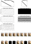
Now you see it. Now you do not. This figure uses the same format as Figure 12 to illustrate the recognition and generation of a short movie of a robin comprising 160 video frames (where the last 32 frames are a repeat of the first 32). The reason there are only 80 timesteps on the x-axis for the level 1 predictive posteriors is that these predictions only pertain to the first of a pair of video frames. The implicit loop has been summarized as a simple orbit through 16 events. In this example, a stimulus was presented for the first four frames and then removed for the subsequent four frames. Despite the absence of precise stimuli, the posterior predictions veridically track the motion of the bird during the missing stimulus.

FIGURE 18

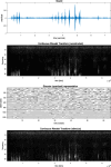
Sound images. This figure shows the training data for structure learning. The lower panel shows the continuous wavelet transform (CWT) of a recording of two crossbill bird calls, where each call comprises a crescendo of short chirps. The CWT is shown as an image of time-frequency responses, that is, the spectral power from 1 to 64 frequency bins, as it evolves over time. Strictly speaking, this is not a continuous wavelet transform because the Gaussian envelope of the Morlet wavelets was fixed at 32 m. As such, this is effectively a short-term Fourier transform between 40 Hz and 4,000 Hz (appropriate for the frequency range of human hearing). The second panel shows the equivalent representation generated from the quantized representation in the third panel. The discrete representation is shown as an image of the probability distributions over singular variates associated with the singular vectors (i.e., time–frequency basis sets) used for discretization. The upper panel shows a sound file generated from the reconstructed CWT.

FIGURE 19

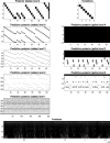
Renormalizing birdsong. This figure uses the same format as Figure 17 but displays the posterior predictions as a continuous wavelet transform (i.e., a time–frequency representation of the spectral power at each point in time). In this example, time–frequency voxels covered four frequency bins and 1,024 time bins, corresponding to approximately 100 m (at a sampling rate of 8,820 Hz). Quantization of the ensuing time–frequency voxels used singular variates with five discrete values for a maximum of 16 singular vectors. This example reports the generation of birdsong after compression to a sequence of eight events. Here, the final event could be followed by any preceding event with equal probability. This follows because there was no recurrence of events in the training data used for structure learning. As a consequence, during generation, events cascade to the eighth event and then transition to a preceding event stochastically. The upper left panel shows the resulting succession of events that produce the posterior predictive sequence of bird calls in the lower panel. When played, the resulting sound file is indistinguishable from a bird emitting a variety of stereotypical calls in a quasi-random sequence.

FIGURE 20

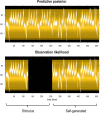
(A) Song recognition. These time–frequency representations reproduce the lower panel of Figure 19 but in the context of an initial stimulus or “prompt,” corresponding to the second call in the training data. These posterior predictions show that the model immediately identified the call and its phase and then continued to generate predictions in accord with its model of successive auditory events. In this example, the stimulus was rendered imprecise (i.e., inaudible) after 16 of the 128 time-frequency voxels were generated. (B) Jazz music. This panel follows the same format as Figure 18; however, here, the recording is of 36 s of jazz piano, comprising approximately 16 bars. The continuous wavelet transform was quantized into 32 frequency bins between 40 Hz and 4,000 Hz (with a fixed Gaussian envelope of 8 m). The (Nyquist) sample rate was twice the highest frequency considered. The time-frequency representation was quantized using time-frequency voxels of four neighboring frequencies and time bins covering approximately 500 m, corresponding to 1/4 of a musical bar. Following renormalization, musical events at the highest (third) level have a duration of 2.24 s; that is, a bar of music.

FIGURE 21

(A) Generating music. This figure follows the same format as Figure 19. In this example, each event corresponds to a bar of music, and the simulation reports the generation of 32 bars under the learned transitions shown on the upper right. Here, the model has learned to generate 8 bars of music until the final bar, after which it re-enters at the first or ninth event to pursue its path through event space. In other words, the model generates stochastically alternating 8-bar musical sequences. This particular generative behavior is a simple consequence of what it has heard during structure learning and subsequent active learning. (B) Musical accompaniment. This panel illustrates the synchronous entrainment of posterior predictions by stimuli. This entrainment can be read as a generalized synchrony (a.k.a., synchronization of chaos) under a shared musical narrative or generative model.

FIGURE 22

Active inference and reinforcement learning. This figure provides two schematics to highlight the difference between active inference and reinforcement learning (i.e., reward-learning) paradigms. Active inference can be read here as subsuming a variety of biomimetic schemes in control theory and the life sciences, such as control as inference (Kappen et al., 2012), model predictive control (Schwenzer et al., 2021), and in neurobiology, motor control theory (Friston, 2011; Todorov and Jordan, 2002), perceptual control theory (Mansell, 2011), the equilibrium point hypothesis (Feldman, 2009), etc. The basic distinction between active inference and reinforcement learning is that in active inference, action is specified by the posterior predictions in outcome modalities reporting the consequences of action. These posterior predictions inherit from policies or plans that minimize expected free energy, namely, Bayesian planning as inference (Attias, 2003; Botvinick and Toussaint, 2012; Da Costa et al., 2020). This kind of planning is Bayes optimal in a dual sense: it conforms to the principles of optimum Bayesian design (Lindley, 1956) and Bayesian decision theory (Berger, 2011) via the maximization of expected information gain and expected value, respectively (where the expected value is defined in terms of prior preferences). Mechanically, this can be expressed as belief updating under a suitable generative model (i.e., planning as inference) to provide posterior predictions that are fulfilled by action (i.e., control as inference). On this view, both belief updating (i.e., perception) and motor control (i.e., action) can be read as minimizing variational free energy. This can be contrasted with reinforcement learning, in which there is an assumed reward function that has a privileged role in updating the parameters of a universal function approximator (e.g., a deep neural network) mapping from inputs (i.e., sensory states) to outputs (i.e., control states). The example of reinforcement learning here uses state-action policy learning based on discounted reward: c.f., Lillicrap et al. (2015) and Watkins and Dayan (1992).

FIGURE 23

Policies and attractors. The upper panels show the first four frames generated by a game engine simulating a simple version of Pong. In this game, the paddle must return a ball that bounces around inside a rectangular box. These images were generated from discrete factors generating (32 × 32) groups of TrueColor pixels where each (12 × 9) factor (i.e., location) could be in five states, corresponding to three parts of the paddle, a ball, or background. In the game engine or generative process, the ball simply bounced around with constant momentum, moving from one location to the next at every time step. The paddle could move in either direction by one location or stay still. A training set of such images (in discretized space) was generated by concatenating sequences of random play that intervened between ball hits. When expressed in terms of probability distributions over quantized states, the ensuing trajectory corresponds to an orbit on a high-dimensional statistical manifold (i.e., simplex). The lower panels illustrate the itinerant nature of this orbit in the space spanned by the first two pairs of singular vectors of the associated time series. The inset provides a magnification of the orbit near the origin of the projection. This inset speaks to a self-similar aspect of the transitions among unique points in this quantized (probabilistic) representation. The number of points corresponds to the unique combination of image features in the training set. These points constitute an attracting set that can be learned under an RGM. Rewarded states or configurations are circled in red, illustrating the fact that there are several paths available for getting from one sparse reward to the next (via unrewarded states).

FIGURE 24

Paths to success. This figure illustrates the transitions among events following structure learning and implicit renormalization of the training sequence. The middle panel shows that the training sequence has been compressed to approximately 256 successive events, with occasional opportunities to switch paths. This follows from the alternative ways in which the paddle can move to reach the same (rewarded) endpoint. The left panel illustrates the paths to hits—that is, rewarded events that include a hit (red circles)—based on the transitions that have been discovered. The requisite paths are shown in white, while the black regions depict events that preclude a hit within the number of time steps along the Y-axis. These can be identified by simply iterating the transitions and asking whether there is an allowable transition from any given state to a rewarded state. This representation suggests that, except for the last few states, there is a path to a reward in six events or fewer (i.e., 6 × 4 = 24 time points). These paths are identified by inductive inference, which assigns a high cost to latent states that preclude a rewarded outcome. The right panel shows these paths at the highest level of events by plotting transitions as a series of arrows in the space spanned by the singular vectors (i.e., principal components) of the graph Laplacian based on the transitions in the middle panel. Each latent state corresponds to a circle, while red circles denote events that entail a hit or reward. This illustrates the itinerant paths available for expert play, moving on orbits that pass through rewarded events. The sequence of events leading to these orbits or attracting latent states can be thought of as an inset, namely, the sequence of events from the initial conditions.

FIGURE 25

(A) Learning expert play. This figure summarizes the results of fast structure learning after exposure to the selected training set. A sequence of 1,024 frames was sampled selectively from 21,280 frames generated with random paddle movement. The ensuing sequence was learned in approximately 18 s on a standard PC. This figure follows the format of previous figures, showing three discovered transitions among certain events, corresponding to the alternative ways in which the paddle moved in the training sequence. This sequence has been summarized in terms of transitions among 233 events. The panel labeled ELBO reports the (negative) variational free energy during continual learning of 512 frames of self-generated play. The red dots correspond to (rewarded) hits, while the colored lines report the ELBO at each level of the RGM. Because the model can only recognize, predict, and thereby realize expert play, the implicit agent never misses the ball (in this example). However, it can learn to become more confident in its (realized) predictions, as evinced by a gradual increase in the ELBO. (B) Breakout. Here, we repeated the analysis using a slightly more complicated game based on Breakout and doubled the number of training frames to 2,048. In this version of Breakout, a reward is recorded whenever the ball hits a row of targets (see lower panels). The row of targets is then removed to expose the underlying row. If a golden target on the final row is hit, the game is reset. Whenever the agent misses a ball or on reset, the paddle is reset to the center, and the ball appears at a fixed height and randomly selected horizontal location around the center. In this example, expert play is confounded by “sticky action,” which means that the movement of the paddle diverges occasionally from the predicted movement. However, the agent recovers quickly and resumes expert play following each miss. This rests on waiting for a recognizable event that is within the attracting set that leads to a reward. As in the previous example, there is a slow increase in confidence with accumulating Dirichlet counts in the likelihood mappings of the RGM. Note that because this game has many more configurations than the previous game of Pong, there are more paths among events; here, there are five such paths (which are shown as discovered transitions by summing over the path dimension of the transition tensor at the final level).

References

1. Adams R. A., Shipp S., Friston K. J. (2013). Predictions not commands: active inference in the motor system. Brain Struct. Funct. 218, 611–643. 10.1007/s00429-012-0475-5 - DOI - PMC - PubMed
1. Alpers G. W., Gerdes A. B. M. (2007). Here is looking at you: emotional faces predominate in binocular rivalry. Emotion 7, 495–506. 10.1037/1528-3542.7.3.495 - DOI - PubMed
1. Angelucci A., Bullier J. (2003). Reaching beyond the classical receptive field of V1 neurons: horizontal or feedback axons? J. physiology 97, 141–154. 10.1016/j.jphysparis.2003.09.001 - DOI - PubMed
1. Attias H. (2003). Planning by probabilistic inference. Proc. 9th Int. Workshop Artif. Intell. Statistics.
1. Ay N., Bertschinger N., Der R., Guttler F., Olbrich E. (2008). Predictive information and explorative behavior of autonomous robots. Eur. Phys. J. B 63, 329–339. 10.1140/epjb/e2008-00175-0 - DOI
LinkOut - more resources