Theoretical and experimental study on traveling wave propagation characteristics of artificial basilar membrane

Abstract

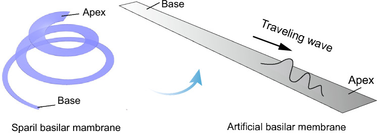
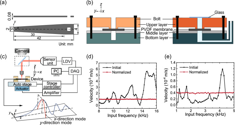
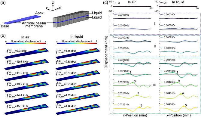
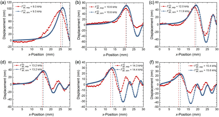
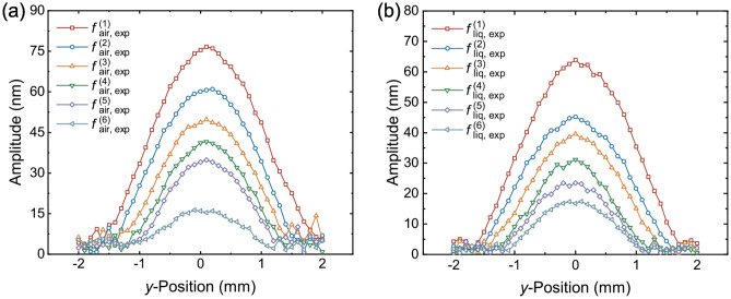
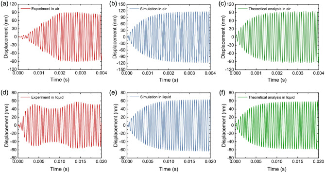
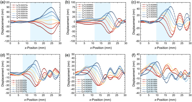
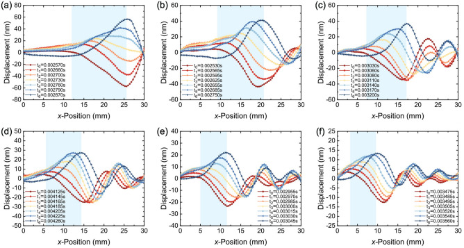
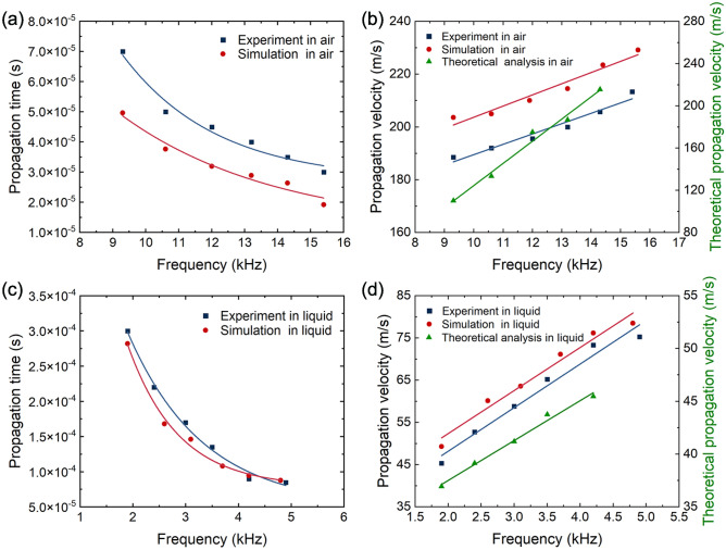
The traveling wave phenomenon in the artificial basilar membrane (ABM) plays a crucial role in the frequency selectivity and electromechanical signal generation of cochlear implants. Continuous measurement of traveling wave propagation remains challenging due to its rapid spatial displacement variation and the requirement for biomimetic conditions in liquid environments. To address this, we developed a laser Doppler optical scanning system with high spatiotemporal resolution, combined with a fixation device replicating cochlear boundary constraints, and successfully captured the traveling wave propagation process. The traveling wave characteristics of the ABM, including propagation time, velocity, frequency selectivity, and local resonance, are revealed. Experimental results indicate that fluid-mass loading and coupling effects significantly reduce the resonance frequency from 9.3-15.4 kHz in air to 1.9-4.9 kHz in liquid and decrease the propagation velocity from 199.20 m/s to 61.78 m/s under our typical experimental conditions. By correlating spatial modes and local resonances with theoretical analysis, we observe that as the resonance frequency increases, the traveling wave propagates faster, reducing propagation delay. The quantification of traveling wave propagation characteristics provides a critical theoretical and experimental foundation for improving the tonotopic accuracy and biological fidelity of cochlear implants.

Keywords: Basilar membrane; Cochlear implant; Frequency selectivity; Traveling wave.

Fig. 1

Schematic illustration of the basilar membrane (BM) and the artificial basilar membrane (ABM). The BM exhibits a spiral geometry with a varying width, and the ABM is designed as a biomimetic model of its planar extension.

Fig. 2

Prototype design, experimental setup, and input energy normalization analysis of the artificial basilar membrane (ABM). (a) Geometry and dimensions of the ABM prototype device. (b) The fixation devices of ABM in air and liquid environments. (c) Overview of the experimental setup. The experimental device of the ABM and the actuator were respectively fixed on the surface and bottom of the automatic stage. The vibration displacement was measured by laser Doppler vibrometer (LDV), and the position of the laser was monitored by a camera. The schematic diagram of the captured traveling wave modes in the x and y directions is illustrated. (d,e) The input velocity normalization results. The response of the maximum velocity at the bottom layer of the fixation device to the input frequency under the initial input voltage (triangle symbols) and normalized voltage (circular symbols) in air (d) and liquid (e) environments, where  V.

Fig. 3

Frequency selectivity analysis of the artificial basilar membrane (ABM) based on numerical simulation and the process of displacement variation. (a) Three-dimensional simulation models of the ABM in air and liquid environments. (b) Numerical simulation results of the displacement distribution of the ABM under different resonance frequencies in air and liquid environments, where is the oscillation mode, envi = air, liq represents the air and liquid environments. Contours represent the relative displacement of each resonance frequency, normalized by the maximum value of the oscillation displacement. (c) The displacement variation process of the ABM obtained experimentally under air and liquid environments at the fourth-order resonance frequency , where = 13.2 kHz and = 3.5 kHz. At t = 0 s, since no oscillation excitation is applied, the displacement is zero. After the oscillation excitation is applied, in the initial stage (I), displacement occurs, but no traveling wave is generated. In the transition stage (II), the traveling wave mode becomes increasingly obvious and the amplitude gradually increases. In the periodic stage (III), the traveling wave is generated and moves cyclically from the basal to the apical region.

Fig. 4

The x-direction modes obtained from experiments (circular symbols) and simulations (triangle symbols) at different resonance frequencies in the air environment when traveling waves reach the resonance positions. The position where the displacement of the first wave peak reaches its maximum value is the resonance position , shown by the dotted line. As the resonance frequency increases, the number of traveling wave peaks increases and the resonance position shifts to the base.

Fig. 5

The x-direction modes obtained from experiments (circular symbols) and simulations (triangle symbols) at different resonance frequencies in the liquid environment when traveling waves reach the resonance positions. The position where the displacement of the first wave peak reaches its maximum value is the resonance position , shown by the dotted line. As the resonance frequency increases, the number of traveling wave peaks increases and the resonance position shifts to the base.

Fig. 6

The y-direction modes of traveling waves on the artificial basilar membrane obtained from experiments in air (a) and liquid (b) environments. The oscillation is induced with each resonance frequency at the resonance y-positions. The amplitudes are all zero near the fixed boundary, and the amplitude is maximum at . The amplitude and slope near the fixed boundary are zero, indicating that the y-direction mode of the traveling wave is the fundamental mode.

Fig. 7

Local resonance at the resonance position at the first resonance frequency in air (a–c) and liquid (d–f) environments. (a,d) are experimental results, (b,e) are simulation results, and (c,f) are theoretical analysis results obtained based on Eq. (10). Local resonance represents the displacement variation over time at the resonance position corresponding to each resonance frequency. The local resonance obtained by experiment, simulation and theoretical analysis is consistent in amplitude and fluctuation time, which verifies the correctness of the resonance frequency and position.

Fig. 8

The propagation process of traveling waves in the air environment. The propagation process starts from when the displacement of the first wave peak is zero and ends at when the first wave peak reaches the resonance position. From to , seven time points are selected to evenly distribute the motion process in the x-direction and characterize the traveling wave propagation. The resonance frequencies are (a) 9.3 kHz, (b) 10.6 kHz, (c) 12.0 kHz, (d) 13.2 kHz, (e) 14.3 kHz, and (f) 15.4 kHz, respectively. The propagation distance of the traveling wave is expressed as the shaded area.

Fig. 9

The propagation process of traveling waves in the liquid environment. The propagation process starts from when the displacement of the first wave peak is zero and ends at when the first wave peak reaches the resonance position. From to , seven time points are selected to evenly distribute the motion process in the x-direction and characterize the traveling wave propagation. The resonance frequencies are (a) 1.9 kHz, (b) 2.4 kHz, (c) 3.0 kHz, (d) 3.5 kHz, (e) 4.2 kHz, and (f) 4.9 kHz, respectively. The propagation distance of the traveling wave is expressed as the shaded area.

Fig. 10

Experimental, simulation, and theoretical results of propagation time and velocity in air (a,b) and liquid (c,d) environments. (a,c) The relationship between propagation time and frequency, and the solid line is the exponential function fitting of the experimental and simulation data. (b,d) The relationship between propagation velocity and frequency, and the solid line is the linear fitting of experimental, simulation and theoretical analysis data.

References

1. Gold, T. & Pumphrey, R. J. Hearing. I. The cochlea as a frequency analyzer. Proc. R. Soc. Lond. Ser. B-Biol. Sci.135, 462–491. 10.1098/rspb.1948.0024 (1948).
1. Reichenbach, T. & Hudspeth, A. The physics of hearing: fluid mechanics and the active process of the inner ear. Rep. Prog. Phys.77, 076601. 10.1088/0034-4885/77/7/076601 (2014). - PubMed
1. White, R. D. & Grosh, K. Microengineered hydromechanical cochlear model. Proc. Natl. Acad. Sci.102, 1296–1301 (2005) http://www.jstor.org/stable/3374424. - PMC - PubMed
1. Inaoka, T. et al. Piezoelectric materials mimic the function of the cochlear sensory epithelium. Proc. Natl. Acad. Sci.108, 18390–18395. 10.1073/pnas.1110036108 (2011). - PMC - PubMed
1. Fowler, E. P. Limited lesions of the basilar membrane. Arch. Otolaryngol.-Head Neck Surg.10, 624–632. 10.1001/archotol.1929.00620090066005 (1929).
Substances
LinkOut - more resources