Air pollution and the number of daily visits of hypertension in northern china: a time-series analysis on generalized additive model

Abstract

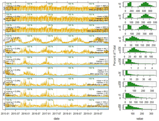
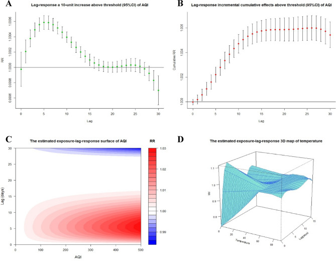
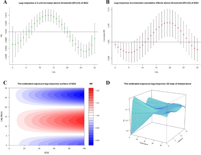
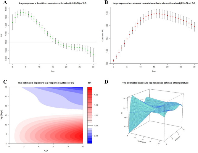
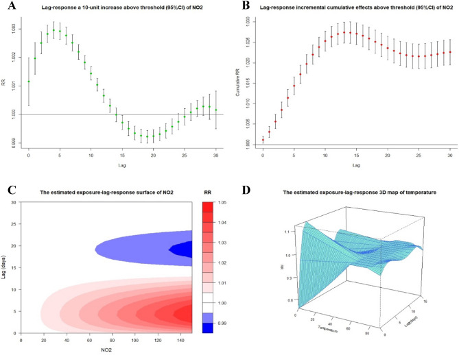
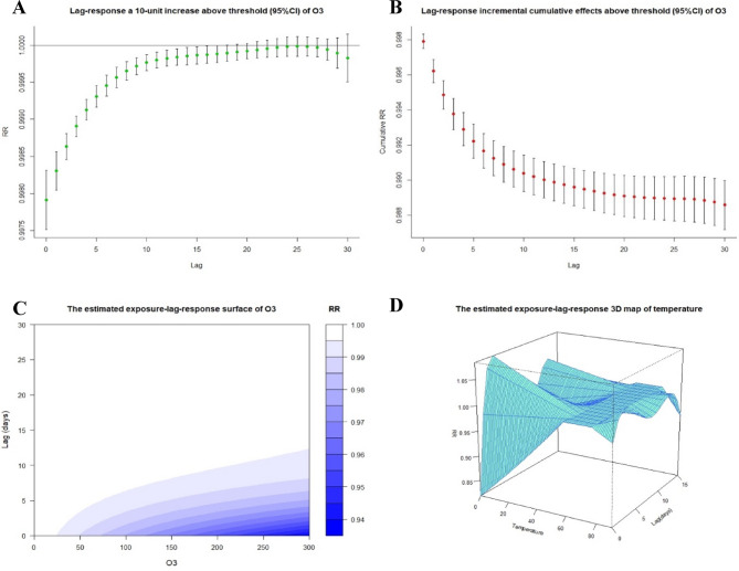
To investigate the correlation between environmental-meteorological factors and daily visits for hypertension in Beijing, China. Daily outpatient and emergency visits for hypertension during January 1st, 2015 and December 31st, 2019 were collected from Capital Medical University affiliated Beijing Shijitan Hospital. We used a time-series generalized additive model and cross-basis to analyze the correlation between atmospheric pollutants, temperature and hypertension emergency visits, with adjustments for time trends, additional meteorological variables, weekday effects and holiday effects. The R 3.6.3 software was engaged to estimate Spearman's correlation coefficients, plot lag-response curves depicting the specific cumulative effects (SCE) and incremental cumulative effects (ICE) of relative risk (RR), alongside the response diagram and three-dimensional diagram of the predicted exposure lag effect. The fitted model was used to forecast the lag RR and 95% confidence interval (95% CI) of SCE and ICE for arbitrary air pollutants at varying concentration degrees. The overall lag-response RR curves for SCE and ICE of PM2.5, PM10, SO2, NO2 and CO were statistically significant. When the concentrations of PM2.5, PM10, SO2, NO2 and CO surpassed certain thresholds, and temperature dropped below 45 °F (with 70 °F as reference value), there was an observed increase in the number of hypertension, accompanied by a time lag effect. Elevated atmospheric concentrations of PM2.5, PM10, SO2, CO and NO2 are significantly correlated with an increase in hypertension-related emergency visits. The peak specific cumulative effects (SCE) and peak incremental cumulative effects (ICE) demonstrating a virtually consistent time lag effect, highlight the imperative for a holistic approach to air pollution management. Additionally, when temperatures fall below 45 °F, there is a notable increase in hypertension visits, accompanied by a lag effect.

Keywords: Air pollution; Environmental-meteorological factors; Generalized additive model; Hypertension; Time-series analysis.

Fig. 1

Time-series plot of daily hypertension visits and daily air pollution concentrations from January 1 st, 2015 to December 31 st, 2019.

Fig. 2

Spearman correlation coefficient matrix graph.

Fig. 3

The overall lag-response RR curves of SCE and ICE associated with every 10-unit increase in the AQI (A, B). The response and three-dimensional diagram of predicted exposure lag effect for AQI (C). The response and three-dimensional diagrams of predicted exposure lag effects for temperature in the model corresponding to AQI (with 70 °F as reference value) (E, F) Note: R² of GAM model is 0.863.

Fig. 4

The overall lag-response RR curves of SCE and ICE associated with every 10-unit increase for PM2.5 (A, B). The response and three-dimensional diagram of predicted exposure lag effect for PM2.5 (C). The response and three-dimensional diagram of predicted exposure lag effect for temperature in the model corresponding to PM2.5 (with 70 °F as reference value) (D). Note: R2 of GAM model is 0.864.

Fig. 5

The overall lag-response RR curves of SCE and ICE associated with every 10-unit increase for PM10 (A, B). The response and three-dimensional diagram of predicted exposure lag effect for PM10 (C). The response and three-dimensional diagram of predicted exposure lag effect for temperature in the model corresponding to PM10 (with 70 °F as reference value) (D). Note: R2 of GAM model is 0.863.

Fig. 6

The overall lag-response RR curves of SCE and ICE associated with every 5-unit increase for SO2 (A, B). The response and three-dimensional diagram of predicted exposure lag effect for SO2 (C). The response and three-dimensional diagram of predicted exposure lag effect for temperature in the model corresponding to SO2 (with 70 °F as reference value) (D). Note: R2 of GAM model is 0.862.

Fig. 7

The overall lag-response RR curves of SCE and ICE associated with every 1-unit increase for CO (A, B). The response and three-dimensional diagram of predicted exposure lag effect for CO (C). The response diagram and three-dimensional diagram of predicted exposure lag effect for temperature in the model corresponding to CO (with 70 °F as reference value) (D). Note: R2 of GAM model is 0.866.

Fig. 8

The overall lag-response RR curves of SCE and ICE associated with every 10-unit increase for NO2 (A, B). The response and three-dimensional diagram of predicted exposure lag effect for NO2 (C). The response and three-dimensional diagram of predicted exposure lag effect for temperature in the model corresponding to NO2 (with 70 °F as reference value) (D). Note: R² of GAM model is 0.865.

Fig. 9

The overall lag-response RR curves of SCE and ICE associated with every 10-unit increase for O3 (A, B). The response diagram and three-dimensional diagram of predicted exposure lag effect for O3 (C). The response diagram and three-dimensional diagram of predicted exposure lag effect for temperature in the model corresponding to O3 (with 70 °F as reference value) (D). Note: R² of GAM model is 0.864.

References

1. Global Burden of 369. Diseases and injuries in 204 countries and territories, 1990–2019: a systematic analysis for the global burden of disease study 2019. Lancet396, 1204–1222 (2020). - PMC - PubMed
1. Marie-Abele, B. et al. Air Pollution and Markers of Coagulation, Inflammation, and Endothelial Function: Associations and Epigene-environment Interactions in an Elderly Cohort. Epidemiology (Cambridge, Mass.). 23, 40–332 (2012). - PMC - PubMed
1. Yuanyuan, C. et al. Associations of Short-term and Long-term exposure to ambient air pollutants with hypertension: a systematic review and Meta-analysis. Hypertens. (Dallas Tex. : 1979). 68, 62–70 (2016). - PubMed
1. You-Jung, C. et al. Short-term effects of air pollution on blood pressure. SCI. REP-UK. 9, 20298 (2019). - PMC - PubMed
1. JH, C. et al. Seasonal variation of effect of air pollution on blood pressure. J. EPIDEMIOL. COMMUN. H. 61, 314–318 (2007). - PMC - PubMed
MeSH terms
LinkOut - more resources