Haploblocks contribute to parallel climate adaptation following global invasion of a cosmopolitan plant

Abstract

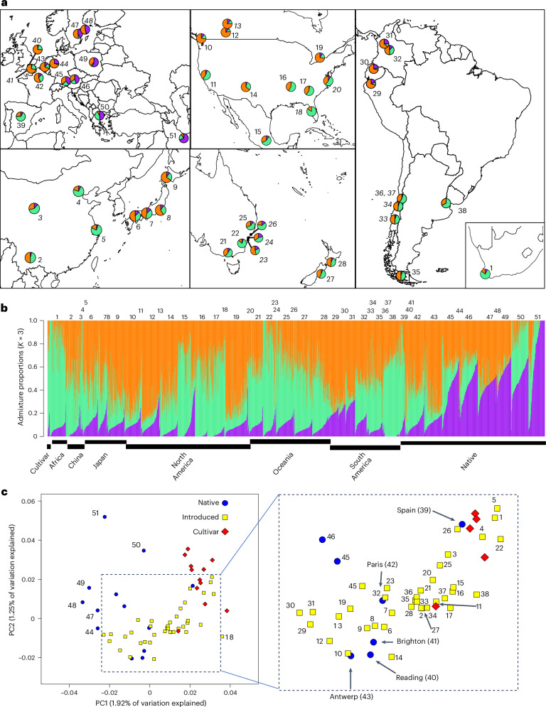
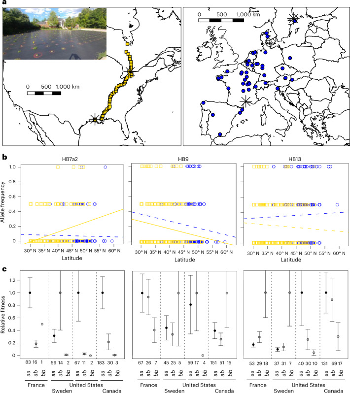
The role of rapid adaptation during species invasions has historically been minimized with the assumption that introductions consist of few colonists and limited genetic diversity. While overwhelming evidence suggests that rapid adaptation is more prevalent than originally assumed, the demographic and adaptive processes underlying successful invasions remain unresolved. Here we leverage a large whole-genome sequence dataset to investigate the relative roles of colonization history and adaptation during the worldwide invasion of the forage crop, Trifolium repens (Fabaceae). We show that introduced populations encompass high levels of genetic variation with little evidence of bottlenecks. Independent colonization histories on different continents are evident from genome-wide population structure. Five haploblocks-large haplotypes with limited recombination-on three chromosomes exist as standing genetic variation within the native and introduced ranges and exhibit strong signatures of parallel climate-associated adaptation across continents. Field experiments in the native and introduced ranges demonstrate that three of the haploblocks strongly affect fitness and exhibit patterns of selection consistent with local adaptation across each range. Our results provide strong evidence that large-effect structural variants contribute substantially to rapid and parallel adaptation of an introduced species throughout the world.

Fig. 1. Population structure across worldwide populations of white clover.

a, NGSadmix ancestries mapped across worldwide sampling. Each pie chart within map inserts reflects the average ancestries (K = 3) from a given wild population with orange, purple and green corresponding to different ancestries. Cultivars are not included. Numbers represent each population; normal typeset indicates population have >30 samples, italics indicates a population has <10 samples. b, Barplots depict ancestry output from the most likely K value (K = 3) for 2,660 individuals. Individuals are organized along the x axis by population sorted by continent, longitude and ancestry values. Numbers above barplots indicate populations from the above map. c, PCA visualizing population structure across ranges. Colour and shape indicate geographic location of each population as shown in the legend. Insert amplifies area of overlap between native and introduced populations. Numbers refer to populations from a and b. The ‘Spain’ point refers to samples from four cities with limited population structure. Source data

Fig. 2. Signatures of structural variants are enriched for patterns of parallel selection across regions where white clover has been introduced.

a, Upset plot depicting outlier windows for native–introduced region contrasts. b, Upset plot depicting windows corresponding to climate adaptation in each range (outliers for XtX statistic and correlations with at least one climate variable). Blue portions of bars in a and b correspond to genomic windows within haploblocks, while black portions of bars represent non-haploblock regions. c, Five haploblocks (putative structural variants indicated by blue bars above the region) identified as outliers on MDS axes summarizing local population structure along chromosomes. Source data

Fig. 3. Haploblocks exhibit molecular signals of selection following introduction.

Empirical P values for enrichment of XtX (an F_ST-like statistic that includes a correction for population structure) in 20-kbp windows across the genome using the WZA within each white clover range. Numbers along the x axis indicate chromosome number. Red points indicate XtX-EAA outliers, windows that are in top 1% of WZA scores for XtX and correlation (Kendall’s Tau) with at least one climate variable. Blue bars indicate haploblock locations. Source data

Fig. 4. Impacts of haploblock variation on fitness across four field common gardens.

a, Experimental design of the transcontinental field experiment. Points represent the 96 populations that were planted into each garden. Black asterisks are the locations of each garden. Insert picture is of the Mississauga, Ontario, Canada, garden. b, Alternative haploblock allele frequency for each individual from European (blue circles) populations or North American (gold squares) pooled across all four common gardens. Regression lines model allele frequency by latitude in Europe (blue) and North America (gold) with solid lines indicating statistically significant (two-sided ANOVA, P < 0.05) latitudinal clines and dash lines indicating non-significant regressions. c, Average relative fitness for each haploblock genotypes where the a allele represents the reference allele and the b allele represents that alternative allele. Numbers directly above genotypes are the number of samples included in each category. Relative fitness was calculated from total seed mass and standardized by the genotype with the highest fitness within each garden. Error bars represent standard error around the mean. Source data

Fig. 5. Associations with fitness and differential expression within haploblocks.

GWAS hits for survival to flowering (triangles) and total seed mass (circles) are plotted above expression ribbons. Each dotted line corresponds to a GWAS analysis within a particular garden (Mississauga, Lafayette, Uppsala or Montpellier) or a GWAS analysis that merged the North American gardens (North America). Hits that either fall within a coding sequence or are within 10 kb of a known homologue are marked with a Greek or mathematical symbol as shown in the legend to the right of each graph. Differential expression ribbons visualize expression patterns for each gene within comparisons between condition (drought versus well-watered), latitude (low versus high) and range (native versus North American). Heatmaps for differential expression for each gene range from downregulated (blue) to upregulated (red). HB7a1, HB7a2 and HB7b are all found on chromosome 7, while HB9 is on chromosome 9 and HB13 is on chromosome 13. The position on chromosomes is indicated beneath differential expression heatmaps for each chromosome. Full descriptions of fitness GWAS hits and differentially expressed genes can be found in Supplementary Tables 3 and 5, respectively. Source data

Extended Data Fig. 1. Population genetic summary statistics across native and introduced ranges.

(a–c) Boxplots compare measures of genetic diversity (π and θ_w) as well as Tajima’s D between native and introduced ranges. Sample size include 13 native populations and 38 introduced populations. (d–f) Boxplots further parse introduced population into individual introduction events. Each point represents the genome-wide average for a single population. Box edges in boxplots represent the interquartile range, center line represents the median, and upper and lower whiskers are the largest value either greater or less than, respectively, 1.5 times the interquartile range. There are 1, 4, 13, 4, 11, 8 and 10 populations included in the Africa, China, Europe, Japan, N. America, Oceania, and South America boxplots, respectively. (g, h) Coalescent reconstructions of effective population size through time as estimated through EPOS. Neither native nor introduced populations exhibit any signatures of bottlenecks following introduction. Instead, most populations show signs of population expansion. Source data

Extended Data Fig. 2. Population structure within and among native and introduced ranges.

a. Weighted pairwise fst within each range, weighted pairwise fst values between native and introduced populations, and weighted pairwise fst values between populations in different introduced ranges. Pairwise fst values are generally low and similar across all worldwide populations. Number of pairwise comparisons included in each boxplot is presented on x-axis below each box. Box edges in boxplots represent the interquartile range, center line represents the median, and upper and lower whiskers are the largest value either greater or less than, respectively, 1.5 times the interquartile range. b–g. Mantel tests for isolation by distance (b-d) and isolation by environment (e-g) across the native range (b,e), North America (c,f) and South America (d,g). Mantel tests are two-sided. Source data

Extended Data Fig. 3. NGSadmix assumed population ancestry mapped across worldwide sampling and cultivars.

a. Barplots depicts ancestry output from K=2,3,4, and 6 K-values. Best K was K=3. Individuals are organized along the x-axis by population sorted by continent, longitude, and ancestry values. b. A map of cultivar origins and NGSadmix assumed ancestries. Each pie chart within map inserts reflects the average ancestries (K=3) from a given wild population (not from cultivars). Pie charts outside the map reflect the ancestry for each cultivar. Arrows indicate the relative locations where wide populations were collected to generate each cultivar. Note that some cultivars were generated from crosses between wild populations from multiple areas. Dotted boxes reflect when the location of the originating wild population is a general location. Note that Durana and Renovation stem from plants collected in Georgia, USA, LA-S1 and Patriot originate from plants in Louisiana, USA and Mississippi, USA respectively, and Pitua is the result of crossing between Spanish and New Zealand accessions. Source data

Extended Data Fig. 4. Genome scan for differentiated regions between Europe and each invasive range.

a. Empirical p-values for enrichment of C₂ (contrast) in 20 kbp windows using the WZA between Europe and each invasive range. Red points indicate the top 1% of WZA scores. Blue bars indicate haploblock locations. b. Overlap between contrast outlier 20 kbp windows and outlier 20 kbp windows within each introduced range (XtX) or across climatic gradients within each range (XtX-EAA). Source data

Extended Data Fig. 5. Climatic correlations with haploblocks and genome-wide variation.

a. Associations between haploblocks and climatic variables from the WORLDCLIM database. b. Overlap between outlier 20kbp XtX windows within each introduced range and outlier windows associated with each climatic variable. Abbreviations: Bio1: Annual Mean Temperature, Bio2: Mean Diurnal Range, Bio8: Temperature in the Wettest Quarter, Bio12: Annual Precipitation, Bio15: Precipitation Seasonality, Bio19: Precipitation in the Coldest Quarter. c–f. Relationships between haploblock allele frequencies and climatic variables. Each point is a single population and is color coded by native or introduced region. Allele frequencies correspond to the frequency of the alternative (non-reference) allele. Source data

Extended Data Fig. 6. Five haploblocks–population-genomic signatures of structural variants.

a. Haploblock clusters for the worldwide population genomics dataset. Three clusters indicative of two homozygous (green and purple) and one heterozygous (orange) structural variant genotypes separate along the first principal component of genetic variation across each haploblock, and furthermore putative heterozygotes show significantly elevated heterozygosity (two-sided Wilcoxon test p < 0.0003 for all heterozygote vs. homozygote comparisons; boxes denote mean ± SEM for each cluster). For better visualization, y-axes have been cropped removing 7, 1, 1, 0 and 6 outlier points for hb7a1, hb7a2, hb7b, hb9 and hb13 plots respectively. Sample sizes (clusters from left to right): HB7a1 1825/250/29, HB7a2 1528/462/111, HB7b 1765/324/15, HB9 1525/441/130, HB13 688/783/633. b. Haploblock clusters are apparent using local PCAs and heterozygosity values derived from SNP data for 109 higher-coverage (~10X) Toronto samples. Colors reflect genotypes assigned from the global dataset. Note that there were no samples genotyped as homozygous for the rare HB7a1 allele in Toronto. Boxes denote mean ± SEM for each cluster. Sample sizes (clusters from left to right): HB7a1 109/9/0, HB7a2 64/41/13, HB7b 80/35/3, HB9 93/22/3, HB13 93/24/1. c. Local patterns of linkage disequilibrium (the second highest value in each 100kb window) corresponding to haploblock regions (blue bars) are present in a random sample of individuals (top triangle; matching sample size of bottom triangle) but absent in samples homozygous for the common haploblock allele (bottom triangle). d. Estimated allele frequencies of each haploblock. Source data

Extended Data Fig. 7. Comparisons of selective signatures within haploblock and non-haploblock windows across the genome.

a. Distribution of WZA 20 kbp window scores for contrasts between Europe and each invasive range for non-haploblock (gray) and haploblock (light blue) windows. b–g. Distribution of XtX statistics and Kendall’s Tau for several climatic variables from the WorldClim dataset for each region. For boxplots, box edges represent the interquartile range, the center line in the box is the median, and the whiskers represent 1.5 times less or greater than the interquartile range. Abbreviations: Bio1: Annual Mean Temperature, Bio2: Mean Diurnal Range, Bio8: Temperature in the Wettest Quarter, Bio12: Annual Precipitation, Bio15: Precipitation Seasonality, Bio19: Precipitation in the Coldest Quarter. EU = Europe, nAM = North America, sAM = South America, OC = Oceania, CN = China, and JP = Japan. Sample sizes (non-haploblock/ haploblock): A: EU-nAM 42694/703, EU-sAM 42679/706, EU-OC 35184/560, EU-CN 42517/696, EU-JP 42788/703; B: 43915/728; C: 44235/731; D: 44099/728; E: 39375/650; F: 44162/727; G: 44257/731. Source data

Extended Data Fig. 8. Associations between fitness variables and haploblock genotypes across four common gardens.

ANOVA results based on a type-III sum-of-squares and two-sided tests. Both survival measures were modeled within a generalized linear model with a binomial distribution and logit link function. Total Seed Mass does not include individuals that did not survive to flowering. Absolute fitness is measured as total seed mass with individuals not surviving to flowering having zero total seed mass. Total seed mass and relative fitness were log+1 transformed to improve model fit. Bold values indicate statistically significant factors at p < 0.05. Source data

Extended Data Fig. 9. Manhattan plots summarizing associations with fitness across haploblocks.

a. Associations between haploblock genotypes with survival to flowering. b. Associations between haploblock genotypes with total seed mass (including zeros for plants that did not survive to flowering). P-values correspond to score statistic (a two-sided test) and are not corrected for multiple comparisons. The Bonferroni corrected significance threshold (horizontal red line) is specific to each haploblock and garden. Gene names are given only for hits landing within coding sequence of annotated genes. Source data

Extended Data Fig. 10. Characterization of the genic content of haploblock regions.

a, b. Histograms summarizing expected numbers of GWAS hits for each haploblock for survival to flowering (a) and total seed mass (b) within the North American common gardens across 160,000 simulations. Observed number of GWAS hits are displayed as vertical red lines. c. Differential expression analysis of RNAseq data within each haploblock. Percentage of genes differentially expressed and absolute expression (log₂FoldChange) is presented between ranges (Europe vs. North America), between Treatments (Well-Watered vs. Dry Down), and between Latitudes (Low vs. High). Values on either side of paratheses for absolute expression are the observed / expected values. Expected values are derived from a two-sided permutation analysis that re-sampled regions from across the genome with replacement. P-values are greater than 0.05 in all cases. Source data

References

1. Pimentel, D., Lach, L., Zuniga, R. & Morrison, D. Environmental and economic costs of nonindigenous species in the United States. BioScience50, 53 (2000).
1. Pimentel, D., Zuniga, R. & Morrison, D. Update on the environmental and economic costs associated with alien-invasive species in the United States. Ecol. Econ.52, 273–288 (2005).
1. Diagne, C. et al. High and rising economic costs of biological invasions worldwide. Nature592, 571–576 (2021). - PubMed
1. Hayes, K. R. & Barry, S. C. Are there any consistent predictors of invasion success? Biol. Invasions10, 483–506 (2008).
1. Catford, J. A. et al. Traits linked with species invasiveness and community invasibility vary with time, stage and indicator of invasion in a long‐term grassland experiment. Ecol. Lett.22, 593–604 (2019). - PubMed
LinkOut - more resources