Cerebellar and subcortical contributions to working memory manipulation

Abstract

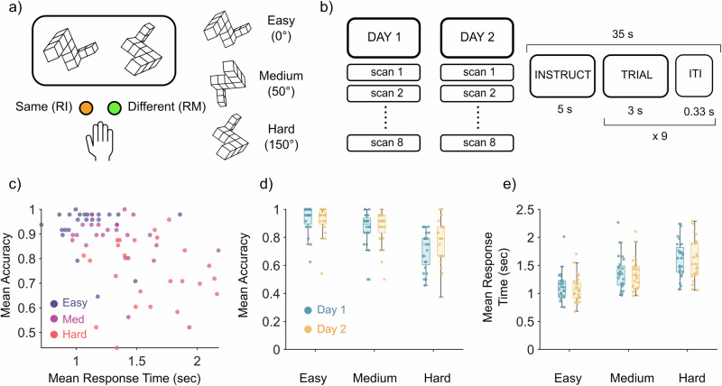
Working memory is critical for manipulating and temporarily storing information during cognitive tasks such as problem-solving. Most models focus primarily on cortical-cortical interactions, neglecting subcortical and cerebellar contributions. Given the extensive connectivity between the cerebellum, subcortex, and cortex, we hypothesize that they contribute distinct, yet complementary, functions during working memory manipulation. To test this, we used functional Magnetic Resonance Imaging (fMRI) to measure blood oxygen-level dependent (BOLD) activity while participants performed a mental rotation task. Our results revealed a distributed network spanning the cortex, subcortex, and cerebellum that differentiates rotated from non-rotated stimuli and correct from incorrect responses. Notably, delayed responses in premotor, subcortical, and cerebellar regions during incorrect trials, suggest that their precise recruitment is crucial for successful working memory manipulation. These findings expand current models of working memory manipulation, revealing the collaborative role of subcortical and cerebellar regions in coordinating higher cognitive functions.

Fig. 1. Mental rotation task and behavioral results.

a Mental rotation stimuli example. Participants respond with two fingers: right middle (RM), right index (RI). Three levels of difficulty based on angles of rotation applied to the stimulus. b Scanning summary with timing of trial. Each participant underwent 2 days of scanning with 8 scans per day. During each scan, the task was performed for 35 s, consisting of 9 trials as laid out. c Scatter plot of mean response time plotted against mean accuracy across all difficulties. Each data point is the mean response time across all trials of that difficulty for a participant. d Mean accuracy across difficulties between each day. Each data point (n = 24) is the mean accuracy of a participant. Center line, median, box limits, upper and lower quartiles. Whiskers, 1.5× interquartile range. e Mean response time across difficulties between days. Each data point (n = 24) is the mean response time of a participant.

Fig. 2. Neuroimaging analysis pipeline.

a Timing of trial (dotted blue line), and estimated timing after convolving with the hemodynamic response function from SPM12 (pink line). Example design matrix, modeling 15 timepoints per condition. Example of the beta coefficients from a single participant using the FIR design matrix, mean BOLD signal colored by a bold line, thinner lines are individual regions (n = 482). b Overview of dimensionality reduction pipeline. First, the data were z-scored and underwent principal component analysis (PCA). Then the data at each timepoint in PCA space was fed into the LDA classifier with a varying number of principal components. c For the final model, we used the first 13 PCs explaining a total of ~44% variance. d Regions valued by their ability to separate easy vs. hard trials (orange = useful for Hard, blue = useful for Easy). e Left: Distribution of Easy and Hard LDA loadings. Right: Loadings of each difficulty across the duration of a trial. Note: Data were not trained on Medium trials. Mean and standard error are plotted (n = 24). f Regions valued by their ability to separate Hard–Correct vs. Hard–Incorrect (orange = biased to Hard–Correct, blue = biased to Hard–Incorrect). g Left: Distribution of Hard–Correct and Hard–Incorrect LDA loadings. Right: Loadings of each response across the duration of a trial. Mean and standard error are plotted (n = 24).

Fig. 3. Effect of task difficulty on regional BOLD dynamics.

a Plotting regions by their loadings on both LDA vectors (n = 482). b Visualizing regions important that separate Hard from Easy, and Hard–Correct from Hard–Incorrect—detailed atlas labels for these regions are in Supplementary data 3 (n = 108). For brain visualizations of the other quadrants, refer to Supplementary Fig. S4. c–e Group average beta coefficients for c Easy, d Medium, and e Hard trials. Each line is a single region; lines are colored by the 7-Yeo resting-state networks for cerebral regions, then the cerebellum, thalamus, hippocampus, basal ganglia, and other subcortical regions as separate groups. f Group average net BOLD response per difficulty. Each dot is a region’s net BOLD response (n = 108). Net BOLD response is calculated by measuring the area between the curve and y = 0, where direction does matter (positive and negative values cancel out). Center line, median; box limits, upper and lower quartiles; whiskers, 1.5× interquartile range. g Estimated linear relationship between net BOLD and task difficulty as measured from generalized linear mixed models after correcting for multiple comparisons (n = 108; false discovery rate Q < 0.05).

Fig. 4. Cross-correlation of corresponding regions between Hard–Correct and Hard–Incorrect.

a Group average beta coefficients for Hard–Correct trials (n = 108). b Group average Beta coefficients for Hard-Incorrect trials (n = 108). c Cross-correlation of corresponding regions between Hard–Correct and Hard–Incorrect. d Cross-correlation of corresponding regions between Easy and Hard trials. a–d Each line represents a single region and is colored by the 7-Yeo resting-state networks for cerebral regions, then cerebellum, thalamus, hippocampus, basal ganglia, and other subcortical regions as separate groups. e Regions (n = 68) that were delayed by 3 s as seen from (c). f Schematic describing the intuition behind the attractor landscape analysis. The analysis estimates the probability that an event will occur (i.e. a specific brain state), and this value is then transformed into the energy requirement for the state to occur—greater energy requirements incur a lower probability, while lower energy requirements incur a higher probability. g Attractor landscape for the delayed regions in Hard-Correct trials (n = 68). h Attractor landscape for delayed regions in Hard-Incorrect trials (n = 68).

References

1. Baddeley, A. & Hitch, G. Working memory. Psychol. Learn. Motiv.8, 47–89 (1974).
1. Camina, E. & Güell, F. The neuroanatomical, neurophysiological and psychological basis of memory: current models and their origins. Front. Pharmacol.8, 438 (2017). - PMC - PubMed
1. Constantinidis, C. & Wang, X.-J. A neural circuit basis for spatial working memory. Neuroscientist10, 553–565 (2004). - PubMed
1. Christophel, T. B., Klink, P. C., Spitzer, B., Roelfsema, P. R. & Haynes, J.-D. The distributed nature of working memory. Trends Cogn. Sci.21, 111–124 (2017). - PubMed
1. Nyberg, L. & Eriksson, J. Working memory: maintenance, updating, and the realization of intentions. Cold Spring Harb. Perspect. Biol.8, a021816 (2016). - PMC - PubMed
LinkOut - more resources