Perceptual clustering in auditory streaming

Abstract

Perception is dependent on the ability to separate stimuli from different objects and causes in order to perform inference and further processing. We have models of how the human brain can perform such causal inference for simple binary stimuli (e.g., auditory and visual), but the complexity of the models increases dramatically with more than two stimuli. To characterize human perception with more complex stimuli, we developed a Bayesian inference model that takes into account a potentially unlimited number of stimulus sources: it is general enough to factor in any discrete sequential cues from any modality. Because the model employs a non-parametric prior, increased signal complexity does not necessitate the addition of more parameters. The model not only predicts the number of possible sources, but also specifies the source with which each signal is associated. As a test case, we demonstrate that such a model can explain several phenomena in the auditory stream perception literature, that it provides an excellent fit to experimental data, and that it makes novel predictions that we experimentally confirm. These findings have implications not just for human auditory temporal perception, but for a wide range of perceptual phenomena across unisensory and multisensory stimuli.

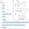
Fig 1. a) Graphical illustration of the clustering problem in causal inference.

As the number of stimuli increases ($1,2,3,4,...$) the number (C) of potential causes increases at the same rate, while the number of combinations of causes that could have generated the stimuli increases according to the number of ways to partition a set of n objects into k nonempty subsets. It is easy to differentiate between the two potential generative structures when there are only two stimuli, but much harder when four stimuli can be created from fifteen different generative structures. b) Example of auditory tones being segregated into one or two streams, using ’galloping’ stimuli similar to [1]. c) Example of a series of potential stimuli with a representative assignment of tones to the streams below. As each tone is presented, the observer reassigns the entire set of tones to streams (1−>12−>123 etc.). The brain has to decide how to assign each tone into an unknown number of streams, a type of clustering problem.

Fig 2. Examples of the likelihood function and CRP prior for a 4th tone given that previous tones [t1,t2,t3] were generated by sources [S1=1,S2=1,S3=2].

This figure illustrates how $\Delta t=(t_i^{on}-t_{i-1}^{off})$ influences the probability of a tone being generated by different sources (as time distance increases, so does the capacity of the source to significantly change its oscillation frequency). It also shows how the CRP prior implements Occam’s Razor by penalizing the probability of a new cluster, and has a “rich gets richer” property by favoring more populated clusters.

Fig 3. a–d) Stimuli used in experiments from [11] (second experiment), highlighting how the speed of presentation affects perception of streams of tones.

Stimuli are shown at the top, bottom are dendrogram tree-plots based on the posterior distribution over clustering. A unique colour is assigned to clusters with more than 50 percent distance from other clusters. a) Slow sequence, ISI 100 ms, tone duration 500 ms, pitch difference [0 4 8 26 30 34 ] semi-tones, tone sequence repeated twice. The posterior mode (the sequence combination with the highest posterior probability) was 111111, i.e. all tones assigned to the same stream. b) Fast sequence, ISI 100ms, tone duration 100 ms (posterior mode 121212). c-d) Example of a galloping stream, from [1], highlighting effect of frequency differences. c) ISI 26.6ms, pitch difference 6 semi-tones (posterior mode 111) d) ISI 26.6ms, pitch difference 20 semi-tones (posterior mode 121). Parameters for this figure (and subsequent figures) were $\alpha =1.44$, $\sigma =40$.

Fig 4. a–b) Stimuli used in experiments from Bregman [26], highlighting the cumulative effect of tones.

Stimuli are shown at the top, and at the bottom are dendrogram tree-plots based on the posterior distribution over clustering. A unique colour is assigned to clusters with more than 50 percent distance from other clusters. a) Short sequence ISI 26.6ms, pitch difference 7 semi-tones, tone sequence repeated twice (posterior mode 111). b) Long sequence ISI 26.6ms, pitch difference 7 semi-tones, tone sequence repeated eight times (posterior mode 121). c-d) Context matters for the clustering of tones. c) Two low tones , two high tones, leading to low tones segregated from high tones (posterior mode 1122); d) While the two low tones have been kept constant, the context of the two other tones now causes them to be clustered separately with the other tones (posterior mode 1212). Long sequence ISI 26.6ms, tone sequence repeated eight times. The modeling parameters were the same as in Fig 3.

Fig 5. Interleaved increasing (uneven numbered tones) and decreasing (even numbered tones) series of tones, ISI 26.6ms.

Same as for human observer the model assigns higher value to a ’bouncing’ percept, where tones [2 4 6 8 10] are clustered together with [13 15 17 19]. Modeling parameters were the same as in Fig 3

Fig 6. a) Behavioural data and model simulations after fitting for four subjects, giving the fraction of trials in which the participant responded ‘2’ for the number of streams perceived.

Axes give the pitch difference for the middle tone and the inter stimulus interval (ISI): the time between the offset of one tone and the onset of the next. b) Model performance on experiment 1 in terms of Evidence Lower Bound (ELBO) for each subject with the CRP model (dark blue), alternative A (red), alternative B (yellow), and alternative C (purple). The black dotted line indicates the performance of a purely random model that assigns 0.5 probability to either response for every condition. Subjects are ordered based on CRP model ELBO values. In order to find a measure of the overall performance of the CRP model we calculated the average relative ELBO between random and perfect model fit (ELBOmin-ELBO)/ELBOmin). This average ELBO proportion is 0.419 for the CRP model, implying a good fit.

Fig 7. D-prime scores as a function of frequency difference. Red bars indicate conditions with a small minimum frequency difference, blue bars indicate conditions with an intermediate minimum frequency difference and green bars indicate conditions with a large minimum frequency difference.

Error bars are $\pm$ 1 standard error

Fig 8. Model performance on experiment 2 in terms of Evidence Lower Bound (ELBO) for each subject with the CRP model (blue), alternative A (red), alternative B (yellow), and alternative C (purple).

The black horizontal dotted line indicates the performance of a purely random model that assigns 0.5 probability to either response for every condition. Subjects are ordered based on CRP model ELBO values. Large negative values indicate poor performance of a model. The average ELBO proportion (calculated as in Experiment 1, where 0 is random and 1 is perfect fit) was 0.127.

Fig 9. Visual representation of a trial with inversion in a 9-9 frequency difference condition.

References

1. van Noorden L. Temporal coherence in the perception of tone sequences. Technische Hogeschool Eindhoven. 1975. https://api.semanticscholar.org/CorpusID:146660865
1. Körding KP, Beierholm U, Ma WJ, Quartz S, Tenenbaum JB, Shams L. Causal inference in multisensory perception. PLoS One. 2007;2(9):e943. doi: 10.1371/journal.pone.0000943 - DOI - PMC - PubMed
1. Shams L, Beierholm UR. Causal inference in perception. Trends Cogn Sci. 2010;14(9):425–32. doi: 10.1016/j.tics.2010.07.001 - DOI - PubMed
1. Wagemans J, Feldman J, Gepshtein S, Kimchi R, Pomerantz JR, van der Helm PA, et al. A century of Gestalt psychology in visual perception: II. Conceptual and theoretical foundations. Psychol Bull. 2012;138(6):1218–52. doi: 10.1037/a0029334 - DOI - PMC - PubMed
1. Aldous DJ. Exchangeability and related topics. Lecture notes in mathematics. 1985. p. 1–198.
LinkOut - more resources