A forward-engineered, muscle-driven soft robotic swimmer

Abstract

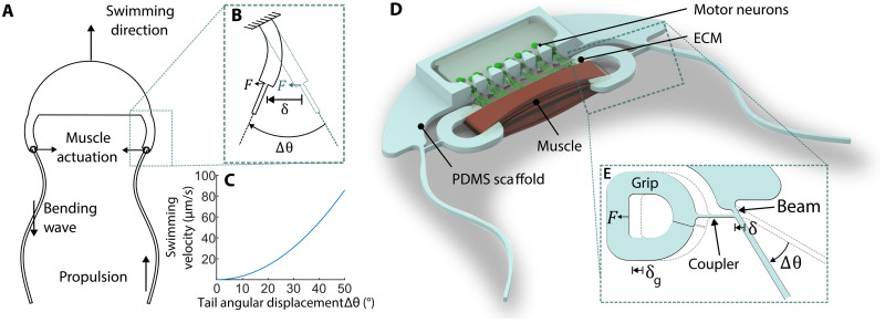
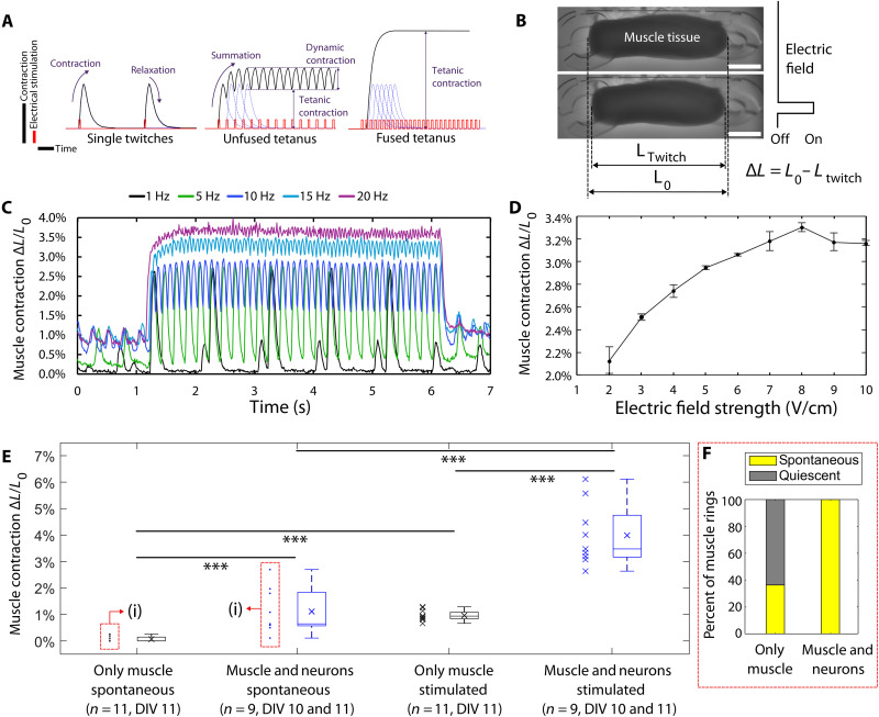
The field of biohybrid robotics focuses on using biological actuators to study the emergent properties of tissues and the locomotion of living organisms. On the basis of models of swimming at small size scales, we designed and fabricated a muscle-powered, flagellate swimmer. We investigate the design of a compliant mechanism based on nonlinear mechanics and its mechanical integration with a muscle ring and motor neurons. We find that within a range of anchor stiffnesses around 1 micronewton per micrometer, the homeostatic tension in muscle is insensitive to stiffness, offering greater design flexibility. The proximity of motor neurons results in a fourfold improvement in muscle contractility. Improved contractility and nonlinear design allow for a peak swimming speed about two orders of magnitude higher than previous biohybrid flagellate swimmers, reaching 0.58 body lengths per minute (86.8 micrometers per second), by a mechanism involving inertia that we verify through flow field imaging. This swimmer opens the door for a class of intermediate-Reynolds number swimmers.

Fig. 1.. Design for the biohybrid swimmer.

The amount of curvature in the swimmer tails is exaggerated in these images to convey the idea of a propagating wave. The optimal swimming speed for a low-Re swimmer occurs when the amount of curvature in the tail is approximately one-quarter of a full wave. (A) Conceptual design highlighting the role of large angular displacement of the base of the tails for generating large amplitude bending waves and propulsion. The relationship between swimming velocity and tail angle change is derived from numerical simulations of the elastohydrodynamic model of the swimmer. (B) A conceptual compliant hinge mechanism, whereby the motion of a muscle contracting and relaxing by distance δ creates an angular displacement Δθ at the base of the tail. (C) Simulated relationship between the angular displacement of the tail and the swimming velocity. (D) Rendering of the biohybrid implementation of the conceptual design. (E) The micromolded PDMS realization of the compliant tail mechanism.

Fig. 2.. Calibration of the PDMS swimmer scaffold.

(A) Schematic of the swimmer scaffold decomposing the overall system into four compliant components. (B) An equivalent spring diagram of the compliant components of the scaffold. The head and the beam contribute to the angular displacement of the tail. (C) Diagram of the setup for calibrating the PDMS scaffold with respect to the stiffness of a tungsten needle (0.43 μN/μm). A hypodermic needle that moves with the tungsten needle acts as a reference. (D) Force-displacement relationships for the components of the scaffold. (E) Calibration curves for approximating the tail angular and translational displacement from position values that can be more accurately quantified from images.

Fig. 3.. Timeline for the biofabrication of the swimmer.

(A) Overall timeline for the biological components. Some preparation steps occur beforehand, including the expansion of a culture of C2C12 myoblasts and the differentiation of mESCs into motor neuron spheroids (see Materials and Methods). (B) Ring molds used for casting the muscle tissue rings. (C) Renderings of the steps involved in mounting the muscle rings on the scaffold. Callouts show tweezer placement necessary to put the muscle into the grips without causing damage. (D) Renderings of the steps involved in mounting the motor neuron spheroids in the head of the swimmer. A hydrophobic paraffin wax substrate causes the ECM to form a bubble around the swimmer. (E) Photograph of the swimmer (scale bar, 2 mm) with callouts showing (F and G) the live bright field (BF) and confocal imaging of the growth of neurites toward the muscle (scale bars, 1 mm) and (H and I) confocal images of sarcomeric α-actinin assembled into sarcomeres localized in the middle of the muscle tissue taken after fixing (scale bars, 25 μm). The neurite GFP signal indicates expression of the Hb9 motor neuron–specific promoter, although other types of neurons are present in the neurospheres due to incomplete differentiation. The photograph of the swimmer was postprocessed by darkening the background around the edge of the PDMS scaffold to help the clear rubber body stand out.

Fig. 4.. Muscle shortening and tonic force during development.

(A) Schematic showing the change in scaffold geometry following removal of the sacrificial supports. (B) Diagram defining how the contraction of the muscle is quantified from bright field images. (C) Force-displacement curves for calculating the tonic tension in the muscle before and after removal of the sacrificial supports. (D and E) Tracking the variation in the muscle length and tonic force in three groups of swimmers. The groups specify whether the sacrificial supports are removed during early, mid, or late differentiation. Statistics indicate the results of one-way analysis of variance (ANOVA) statistical tests comparing the percent of initial lengths of the muscle of the three groups (**P < 0.01; *P < 0.05). For DIV 6 and 9, statistics reflect length measurements taken 1 hour after the removal of the sacrificial supports. By DIV 9, after cutting the sacrificial supports on the last group of samples, large variation among the muscle lengths contributes to the groups being indistinct from one another (P > 0.05 by one-way ANOVA). Insets show the change in force following the removal of the sacrificial supports on DIV 6 and 9. Exponential curve fits give approximate time constants of 4.5 and 5.8 hours for recovery of the force during the 24 hours after release.

Fig. 5.. Characterization of the spontaneous and evoked contractility of the muscle tissues.

(A) Nomenclature used to describe muscle contraction at different stimulation frequencies. (B) Schematic defining how muscle contractility is measured with respect to the resting length of the muscle. (C) Variation in the muscle contractility and dynamics with increasing frequency for a typical swimmer. Low-amplitude spontaneous twitches (~1%) can be seen interspersed with the evoked spikes. Measurements are with respect to the length of the muscle before any stimulation occurred, so the offset at the start of higher frequencies is persistent tetanic contraction. (D) Variation in peak contractility with increasing electrical field strength for a typical swimmer (n = 4, means ± SD). (E) Comparison of the spontaneous and evoked contractility (stimulation, 3 V/cm) of swimmers with and without the inclusion of motor neurons. Statistics refer to t tests assuming independent samples (***P < 0.001). Individual measurements are shown beside their corresponding box plots. “x” annotations indicate the mean of each group. (F) The percentage of muscles in each group that exhibited any spontaneous twitching at the time of the experiment. The highly significant comparison between the spontaneous twitching activities of the two groups includes quiescent, muscle-only swimmers. If instead these are disregarded, then the spontaneous contractility of the groups is not significantly different (P > 0.05).

Fig. 6.. Swimming position tracking and analysis.

(A) Diagram of the template tracking method employed to quantify the swimmer’s position and muscle contraction waveforms. (B) 2D projection of the path of a point on the head of the swimmer before (red) and during (blue) 4-Hz electrical stimulation. (C) The corresponding stimulation, grip displacement, and position of the swimmer during the 4-Hz electrical stimulation. The position is taken by projecting the swimmer’s path onto the direction of travel. Before stimulation, the swimmer drifts with a small velocity. This is attributed to currents in the dish caused by air movement at the free surface and vibrations. Because features normal to the plane of the swimmer scaffold, such as the side of the neuron holder, are visible in microscope recordings, we infer the swimmer is floating with a nonzero angle of attack. When the muscle contracts, the projected length of these features is observed to change as the swimmer pitches forward and backward (fig. S3B). An estimate from these motions gives that the swimmer sits at 16° from the plane of the microscope and pitches 1° to 2° every time the muscle twitches (fig. S3C).

Fig. 7.. Swimming waveforms for a high performing swimmer.

(A) x-y coordinate plots for the swimming trajectory at multiple frequencies. (B) Electrical stimulation waveforms (3 V/cm, 10-ms pulse width). (C) Muscle contraction measured from motion of $x_3$ , the junction between the grip and the coupler. Inset: Grip velocity measured from the attachment of the muscle x₄. (D) Swimmer displacement projected along the swimming trajectory. At frequencies of ≥8 Hz, the onset and relaxation of tetanus give the position waveform a distinct sawtooth shape. (E) Aggregated time-averaged swimming velocities for all swimmers at each frequency. Circled data correspond with the example swimmer presented in (A) to (D). (F to H) Nondimensionalization of the swimmer dynamics with time constant τ = 2.8 s for each of the cases. Background colors refer to time windows in (D).

Fig. 8.. Comparison between experimental swimmer velocities and predictions from our low-Re model.

(A) Aggregated swimming velocities and tail angular displacement amplitudes across all samples (n = 6) compared against regions corresponding to low-Re model predictions generated with the indicated frequencies, tail angle changes, and drag coefficients. Tail angular displacement amplitudes correspond with the dynamic contraction (Fig. 5C) of the input waveform, excluding tetanus contraction. Simulations are run using experimental muscle contractions waveforms as the model inputs. Inputs are scaled to achieve the associated tail angular displacement amplitude. Red circle annotations indicate whether a datum corresponds with a frequency, which induces unfused tetanus in the muscle. (B) Comparison of experimental and predicted swimmer velocities at multiple stimulation frequencies for a single swimmer. The predicted swimming velocities are generated using the experimental muscle contraction for this swimmer as inputs to the simulation.

Fig. 9.. Particle streak visualization of a flow regime transition due to increasing tail angular displacement amplitude and increasing grip velocity.

(A) Schematic for reproducing the flow field of the swimmer tail using a micromanipulator. (B) Example trapezoidal waveforms by the micromanipulator at different speeds and constant peak displacement, overlaid on a waveform of grip displacement produced by a muscle (taken from Fig. 5C for 1-Hz stimulation, n = 4, means ± SD). (C) Box plot of the grip velocities observed during swimming of the six for stimulation frequencies between 0.5 and 5 Hz (n = 36). Grip velocity values are calculated as the average over all contractions of a muscle at a given frequency while swimming. (D) Example particle streak images on either side of the transition corresponding to grip speeds of 180 and 2300 μm/s and maximum angular displacements of 18.5° and 19.8°, respectively. Scale bars, 1 mm. Callouts show example streaks and higher-resolution positional data of the corresponding beads collected using template matching. Units are in micrometers. (E) Quantification of the change in the flow dynamics based on the time-averaged velocity of beads in the direction of the tail (n = 7, means ± SD). Asterisk (*) indicates region corresponding to our experimental swimming results for stimulation frequencies between 0.5 and 5 Hz. (F) Reproduction of the data in Fig. 8A restricted to stimulation frequencies between 0.5 and 5 Hz with corresponding average values of the grip velocity. Grip velocity values are taken as the average over all contractions of a muscle at a given frequency.

References

1. Webster-Wood V. A., “ It’s alive! From bioinspired to biohybrid robots,” in Robotics in Natural Settings. CLAWAR 2022. Lecture Notes in Networks and Systems, Cascalho J. M., Tokhi M. O., Silva M. F., Mendes A., Goher K., Funk M., Eds. (Springer, 2023), vol. 530, pp. 4.
1. Desatnik R., Patterson Z. J., Gorzelak P. I., Zamora S. I., LeDuc P., Majidi C., Soft robotics informs how an early echinoderm moved. Proc. Natl. Acad. Sci. U.S.A. 120, e2306580120 (2023). - PMC - PubMed
1. Mestre R., Patiño T., Sánchez S., Biohybrid robotics: From the nanoscale to the macroscale. Wiley Interdiscip. Rev. Nanomed. Nanobiotechnol. 13, e1703 (2021). - PubMed
1. Filippi M., Yasa O., Giachino J., Graf R., Balciunaite A., Stefani L., Katzschmann R. K., Perfusable biohybrid designs for bioprinted skeletal muscle tissue. Adv. Healthc. Mater. 12, 2300151 (2023). - PMC - PubMed
1. Filippi M., Mekkattu M., Katzschmann R. K., Sustainable biofabrication: From bioprinting to AI-driven predictive methods. Trends Biotechnol. 43, 290–303 (2025). - PubMed
LinkOut - more resources