Sub-nanosecond all-optically reconfigurable photonics in optical fibres

Abstract

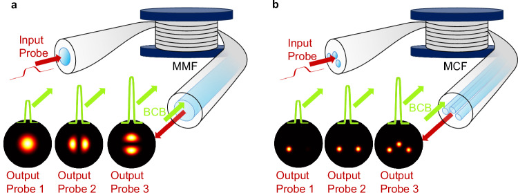
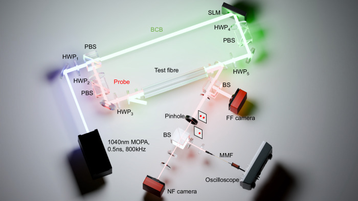
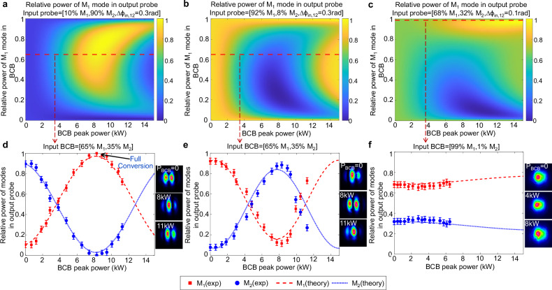
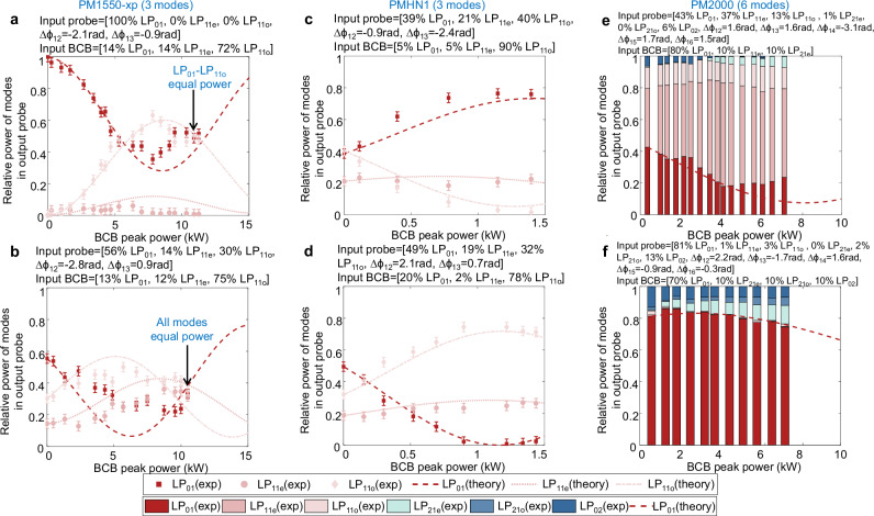
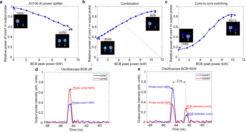
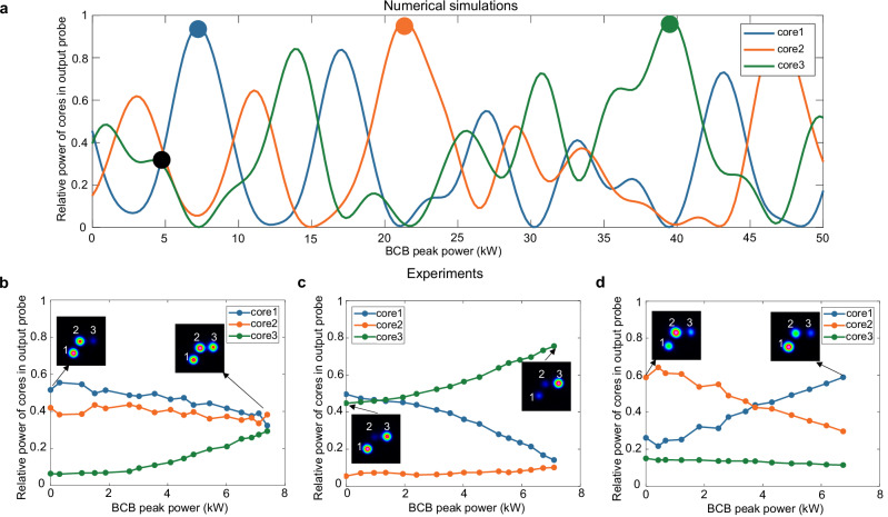
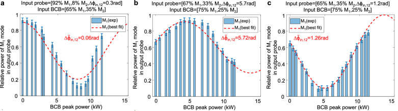
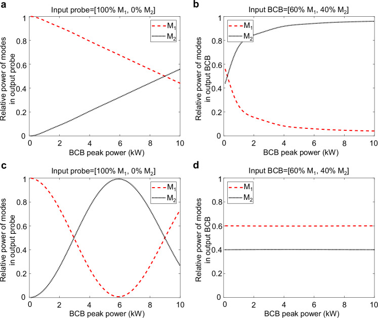
Reconfigurable photonic systems provide a versatile platform for dynamic, on-demand control and switching. Here we introduce an all-optical platform in multimode and multicore fibres. By using a low-power probe beam and a counter-propagating control beam, we achieve dynamic control over light propagation within the fibres. This setup ensures simultaneous phase-matching of all probe-control beam four-wave mixing interactions, enabling all-optical reconfiguration of the probe modal state by tuning the control beam power. Key operations such as fully tuneable power splitting and mode conversion, core-to-core switching and combination, along with remote probe characterization, are demonstrated at the sub-nanosecond time scale. Our experimental results are supported by a theoretical model that extends to fibres with an arbitrary number of modes and cores. The implementation of these operations in a single platform underlines its versatility, a critical feature of next-generation energy-efficient photonic systems. Scaling this approach to highly nonlinear materials could underpin photonic programmable hardware for optical computing and machine learning.

Fig. 1. Illustration of all-optically reconfigurable photonics in optical fibres.

a A low-power probe beam (red colour) and a high-power counter-propagating backward control beam (BCB, green colour) are injected at the two opposite ends of a multimode fibre. The BCB is coupled over a suitable combination of modes. A specific output probe on demand can be obtained by solely adjusting the BCB power. In this example, 3 different BCB intensities lead to an output probe coupled over 3 distinct fibre modes (see Output Probe 1, 2, 3). b Same as panel a, but in the case of a multicore fibre with 3 cores. In this example, by tuning the BCB intensity, the output probe is either fully readdressed over a single core (Output Probe 1), or equally split over 2 (Output Probe 2) or 3 cores (Output Probe 3). The ability to manipulate the probe can be exploited to implement power splitters, mode converters and core-to-core switchers with all-optical reconfiguration at the sub-nanosecond scale.

Fig. 2. Schematic of the experimental setup.

The input probe and BCB are split from a master oscillator power amplifier (MOPA) and coupled to the opposite ends of the test fibre. The MOPA delivers 0.5 ns pulses at a central wavelength of 1040 nm and with peak power up to 30 kW (12 W average power at 800 kHz repetition rate), therefore enabling a significant level of nonlinearity in the fibres under test. Polarisation beam splitters (PBS) and half-wave-plates (HWP_1–5) are used to tune independently the input probe and BCB power and polarisation. A near-field (NF) and a far-field (FF) camera measure the near and far field images used in our mode decomposition algorithm. The field at the output of each core of MCFs can be isolated via a pinhole and its temporal dynamic is monitored at the oscilloscope. SLM = spatial light modulator; BS = beam splitter.

Fig. 3. Tuneable mode manipulation. Results in a bimodal fibre.

This fibre is 0.4 metre long and supports one even mode M₁ and one odd mode M₂ (see Supplementary Information 1). a–c Theoretical 2D maps of the output probe mode distribution computed from Eq. (4). The maps show the output probe power fraction coupled to mode M₁ versus the BCB total peak power (horizontal axis) and BCB mode distribution (vertical axis, indicating the fraction of BCB power coupled to mode M₁). These maps indicate how to set the BCB in order to manipulate the output probe, ensuring it reaches the desired mode distribution. The maps correspond to 3 examples with different input probe mode states, which are reported at the top of each panel. For example, in panel a the input probe mode state is characterised by 10% power on mode M₁, 90% on mode M₂, and a relative phase $\mathrm{\Delta }{\mathrm{\varphi }}_{in,12}$ between the two modes of 0.3 rad. d–f. Experimental (exp) and theoretical (theory) results for the same input probe mode states as panels (a–c), but with a fixed BCB mode distribution (indicated at the top of each panel and corresponding to the red-dashed lines in panels (a–c)). Arbitrary output probe mode distribution can be achieved by tuning the BCB power. Specifically, in panel (d), full conversion to mode M₁ is achieved when the BCB peak power is ~ 8 kW (3.2 W average power). In contrast, the BCB in f is configured such that it results in almost no variation of the output probe mode distribution. The insets in panels (d–f) show the far-field intensities of the output probe for different values of BCB peak power P_BCB. Error bars of ±3% are added to the measured relative power of each mode, which represents the estimated uncertainty of our mode decomposition algorithm.

Fig. 4. Tuneable mode manipulation. Results in various commercially available three- and six-mode fibres.

Experimental (exp) and theoretical (theory) results are shown for different combinations of input probe and BCB mode distributions (indicated at the top of each panel) in a three-mode PM1550-xp, a three-mode PMHN1, and a six-mode PM2000 (all 0.4 m long). The six panels illustrate distinct cases of probe reconfiguration. Error bars of ±3% indicate the uncertainty in the measured relative power of each mode. Note that panels (a–d) use line plots as they involve only three modes. In panels (e, f) where six modes are involved, a bar chart is used instead to prevent excessive visual clutter. (a, b). Results in PM1550-xp fibre; (c, d). Results in PMHN1 fibre; (e, f). Results in PM2000 fibre.

Fig. 5. Tuneable reconfiguration in dual-core fibre.

Three different instances are shown. The insets show the near-field intensities of the output probe at each core. a The input probe launch condition is optimised such that the output probe power is entirely in core 1 when the BCB is off (power ratio core1/core2 = 100/0). After having appropriately fixed the BCB mode state, we increase the BCB peak power from 0 to 9 kW (0 to 3.6 W average power). We then observe that the core-to-core power ratio of the output probe transitions gradually from 100/0 to 50/50, enabling an all-optical, fully tuneable X/(100 - X) power splitting. b Differently from panel a, in this case the output probe core distribution is relatively uniform when the BCB is off (power ratio core1/core2 = 35/65). The output probe is then progressively redirected into core 1 as the BCB power increases, achieving an all-optically controlled combination. At 11 kW of BCB peak power, 92% of the output probe power is in core 1 (power ratio core1/core2 = 92/8). We estimate that full combination (100/0) could be achieved at ~14 kW peak BCB power (not available). c In this example, the output power ratio goes from 15/85 when BCB is off to 85/15 when the BCB peak power is ~10 kW. Full switching (0/100 to 100/0) could be achieved with ~18 kW BCB peak power (not available). d Temporal evolution of output probe power at the two cores measured by the oscilloscope when the BCB is off (power ratio core1/core2 = 35/65). e Temporal evolution of output probe power at the two cores measured by the oscilloscope at 5 kW BCB peak power. The power ratio shifts to 65/35. The oscilloscope also detects the BCB reflection, with the 2 ns delay corresponding to the time of flight of light in the fibre.

Fig. 6. Tuneable reconfiguration in three-core fibre.

Our ability to implement all-optical probe reconfiguration extend to fibres with more than 2 cores. This figure illustrates all-optical operations in a 0.4 m long TCF. The insets show the near-field intensities of the output probe at each core. a Output probe core distribution simulated via Eqs. (1) and (2), with linear and nonlinear coefficients estimated from the fibre parameters (see Supplementary Information 1). In this simulation, the BCB mode state is as follows: 5% of power in mode 1, 30% in mode 2, 65% in mode 3, and all modes in-phase. The probe power can be arbitrary low. By adjusting the BCB peak power from 0 to 50 kW we can either equalise the output probe power in the 3 cores (see black spot) or combine most of the output probe power in core 1 (blue spot), core 2(red spot) or core 3 (green spot). b–d Experimental results in the TCF. Each panel corresponds to different launch conditions of the input probe. In each case, the BCB is optimised to achieve relevant operations for a BCB peak power of ~7 kW (i.e., 2.8 W average power, the maximum we are able to couple into the TCF). In panel b, the output probe is almost equally split across the 3 cores. In panel c, the probe is mainly redirected to a single core (core 3). In panel d, we achieve power swapping between core 1 and core 2.

Fig. 7. Remote characterisation of the input probe.

Experimental results (bars) and corresponding best theoretical fits (red-dashed lines) showing the output probe power fraction coupled to mode M₁ versus BCB peak power in a 0.4-m long bimodal fibre (DCF, see Supplementary Information 1). Panels (a–c) correspond to different input probe mode states and BCB mode distributions, measured experimentally and reported on the top of each panel. The best theoretical fit is calculated from Eq. (4), assuming the same input probe and BCB relative powers and optimising the input probe relative phase to minimise the least squares difference with experimental data. Note that in all the 3 cases the estimated optimal least-squares value $\mathrm{\Delta }{\tilde{\mathrm{\varphi }}}_{in,12}$ (0.06 rad, 5.72 rad, 1.26 rad in panels (a–c) respectively) is close to the measured $\mathrm{\Delta }{\mathrm{\varphi }}_{in,12}$ (0.3 rad, 5.7 rad, 1.2 rad in panels (a–c) respectively). This demonstrates our ability to detect from remote the relative phase of the input probe modes by analysing the output probe response to the BCB. Note that the larger error in panel (a) is due to the large power imbalance among the two input probe modes (92% and 8%, respectively).

Fig. 8. Illustration of linear and nonlinear probe regimes (a–b).

Mode distribution of the output probe (a) and output BCB (b) versus the BCB peak power when the probe is in a strong nonlinear regime (peak power fixed to 10 kW). The output probe is asymptotically attracted to the mode state orthogonal to the input BCB, and vice versa. c, d Mode distribution of the output probe (c) and output BCB (d) versus the BCB peak power when the probe is in linear regime (peak power fixed to 10 mW). The output probe mode distribution oscillates sinusoidally as a function of the BCB power, whereas the BCB mode distribution is unchanged.

References

1. Digonnet, M. J. Rare-earth-doped fiber lasers and amplifiers, revised and expanded. (CRC Press, Boca Raton, 2001).
1. Stolen, R. H. & Bjorkholm, J. E. Parametric amplification and frequency conversion in optical fibers. IEEE J. Quantum Electron18, 1062–1072 (1982).
1. Slavík, R. et al. All-optical phase and amplitude regenerator for next-generation telecommunications systems. Nat. Photon.4, 690–695 (2010).
1. Morioka, T. & Saruwatari, M. Ultrafast all-optical switching utilizing the optical Kerr effect in polarization-maintaining single-mode fibers. IEEE J. Sel. Areas Commun.6, 1186–1198 (1988).
1. Fatome, J., Pitois, S., Morin, P. & Millot, G. Observation of light-by-light polarization control and stabilization in optical fiber for telecommunication applications. Opt. Express18, 15311–15317 (2010). - PubMed
LinkOut - more resources