The neural basis of species-specific defensive behaviour in Peromyscus mice

Abstract

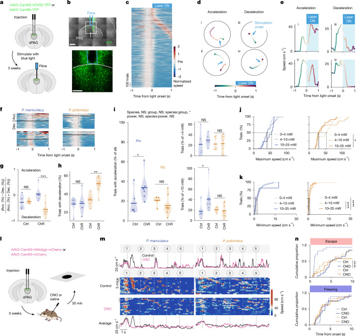
Evading imminent threat from predators is critical for animal survival. Effective defensive strategies can vary, even between closely related species. However, the neural basis of such species-specific behaviours remains poorly understood^1-4. Here we find that two sister species of deer mice (genus Peromyscus)⁵ show different responses to the same looming stimulus: Peromyscus maniculatus, which occupies densely vegetated habitats, predominantly escapes, whereas the open field specialist, Peromyscus polionotus, briefly freezes. This difference arises from species-specific escape thresholds, is largely context-independent, and can be triggered by both visual and auditory threat stimuli. Using immunohistochemistry and electrophysiological recordings, we find that although visual threat activates the superior colliculus in both species, the role of the dorsal periaqueductal grey (dPAG) in driving behaviour differs. Whereas dPAG activity scales with running speed in P. maniculatus, neural activity in the dPAG of P. polionotus correlates poorly with movement, including during visually triggered escape. Moreover, optogenetic activation of dPAG neurons elicits acceleration in P. maniculatus but not in P. polionotus, and their chemogenetic inhibition during a looming stimulus delays escape onset in P. maniculatus to match that of P. polionotus. Together, we trace species-specific escape thresholds to a central circuit node, downstream of peripheral sensory neurons, localizing an ecologically relevant behavioural difference to a specific region of the mammalian brain.

Fig. 1. Evolution of defensive behaviour in ecologically distinct Peromyscus species.

a, Phylogenetic relationship of three focal Peromyscus species with representative photographs of their natural habitat. Image credit: Aimee Tomcho (P. leucopus habitat), Yu Man Lee (P. maniculatus habitat), Hopi Hoekstra (P. polionotus habitat). b, Schematic representation of the sweep–looming stimulus. c, Defensive response of Mus musculus (C57Bl6 strain) during the sweep–looming stimulus. Rows represent individual trials (n = 14 mice, tested twice). Trials are sorted by escape onset during the looming stimulus, with earliest on top. Speed is indicated by a colour gradient. d, Representative movement trajectories of individual mice (n = 10) of P. leucopus, P. maniculatus and P. polionotus during 0.4 s before stimulus onset (left), during sweeping (middle) and during looming (right). Time is indicated by a colour gradient. e, Defensive response of Peromyscus species during the sweep–looming stimulus. Rows represent individual mice (P. polionotus, n = 26; P. maniculatus, n = 29; P. leucopus, n = 28). Trials are sorted by escape onset during the looming stimulus, with earliest on top. Speed colour gradient is the same as in c. Three bars above each raster plot indicate the time period of the trajectories shown in d, and for looming are centred on the peak mean speed of each species. Line plots represent mean speed ± 95% confidence interval (CI); horizontal shaded lines represent the 95% confidence interval of mean speed averaged across the 60 s before stimulus onset.

Fig. 2. Escape threshold differences underlie species-specific behaviour.

a, Left, behavioural response to five repetitions of visual threat of varying intensity (looming contrast: 32%, 72% or 100%). Rows represent individual mice of P. maniculatus (left) and P. polionotus (right). Trials are sorted by latency to escape threshold. Right, proportion of individual mice of P. maniculatus and P. polionotus showing escape (top) and freezing (bottom) across these and additional contrast levels (far right; escape, 32% contrast P = 0.685, 55% contrast P = 4 × 10⁻⁴, 72% contrast P = 2 × 10⁻⁷, 86% contrast P = 9 × 10⁻⁴, 100% contrast P = 0.052; freezing, 32% contrast P = 0.615, 55% contrast P = 4 × 10⁻⁴, 72% contrast P = 2 × 10⁻⁷, 86% contrast P = 0.002, 100% contrast P = 0.0177). b, Cumulative proportion of individual mice showing escape during 100% contrast looming stimulus (latency, P = 0.009; proportion, P = 0.052). c, Cumulative percentage of escaping mice that either escaped without first freezing (solid line) or that first froze and then transitioned to escape (dashed) (P = 0.006). d–f, Raster plots and cumulative proportion of individual mice showing escape and freezing during a single looming stimulus (100% contrast) in the presence of hut (d; escape, P = 4 × 10⁻⁴; freezing, P = 0.007), in the absence of hut (e; escape, P = 2 × 10⁻⁵; freezing, P = 0.009), and during a sound frequency upsweep (f; escape, P = 0.005; freezing, P = 5 × 10⁻⁴). Two-sided chi-squared test (proportion, cumulative proportion and cumulative percentage), two-sided Kolmogorov–Smirnov test (escape onset distribution). Pm, P. maniculatus; Pp, P. polionotus. *P < 0.05; **P < 0.01; ***P < 0.001; ****P < 0.0001; NS, not significant.

Fig. 3. Differential activation of dPAG neurons during escape behaviour.

a, Schematic of behavioural assay. Midbrain regions of interest: deep medial superior colliculus (dmSC) (orange) and dPAG (green). Adapted from Allen Mouse Brain Atlas (https://mouse.brain-map.org and https://atlas.brain-map.org). b, Mean speed during escape of P. maniculatus (P = 0.001) and P. polionotus (P = 0.001) (looming: P. maniculatus n = 13, P. polionotus n = 38; control: P. maniculatus n = 6, P. polionotus n = 4). Filled circles indicate samples stained for FOS. c, Representative images of FOS expression in dmSC and dPAG. Scale bars, 500 μm. Dashed white boxes indicate regions shown in d,e. dlSC, deep lateral superior colliculus. d,e, Images (left) and quantification (right) of FOS⁺ cells in the dmSC (d) and dPAG (e) of control and looming-exposed mice (looming, P. maniculatus, n = 9; P. polionotus, n = 15; controls, n = 6; dSC: P. maniculatus, P = 2 × 10⁻⁶, P. polionotus, P = 0.003; dPAG: P. maniculatus, P = 6 × 10⁻⁶, P. polionotus, P = 0.213). Scale bars, 50 μm. f, Quantification of FOS⁺ cells in dPAG as a function of number of FOS⁺ cells in dmSC of looming-exposed mice (species, P = 0.007; dmSC, P = 0.004). g, Number of FOS⁺ cells in dPAG as a function of mean speed during escape in looming-exposed mice (species, P = 3 × 10⁻⁴; speed, P = 0.001). Encircled points indicate samples selected for analysis in h,i. h, Representative images of FOS (top), GAD1 (middle) and merged (bottom) staining in the dPAG. Yellow arrowheads indicate double-labelled cells. Scale bars, 50 μm. i, Proportion of FOS⁺ excitatory (VGluT2 (also known as Slc17a6); top) and inhibitory (Gad1; bottom) dPAG neurons in subset of control and strongly escaping mice. Model fit and 95% confidence interval are shown. Points represent tissue sections (VGluT2, looming: P. maniculatus n = 6, P. polionotus n = 8, controls: n = 9; Gad1, looming: P. maniculatus n = 7, P. polionotus n = 8, controls: n = 9), collected from three mice per species (VGluT2, P. maniculatus, P = 0.003, P. polionotus, P = 0.014; Gad1, P. maniculatus, P = 0.001, P. polionotus, P = 0.228). Statistical significance evaluated with mixed-effects models.

Fig. 4. Species-specific encoding of locomotion in the dPAG.

a, Schematic of immersive set-up. b, Running speed (top) and escape onset (bottom) during triple loom stimuli. P. maniculatus, n = 6 mice; P. polionotus, n = 4. c, Concatenated responses of 100 cells per area for trials with highest stimulus correlation (column 1–3) and one escape trial (last column). d, Example cells in the sSC, dSC and dPAG during stimuli without (left) and with (middle) escape, and corresponding Spearman coefficients. Right, behavioural selectivity index (SI) for each neuron. Vertical lines indicate median, horizontal lines represent interquartile range and diamonds show the mean. Squares indicate example cells. e, Cumulative distributions (left; dPAG–dPAG P = 3 × 10⁻¹⁰; P. maniculatus sSC–dPAG P = 0.012, dSC–dPAG P = 0.021) and quantification (right; sSC–dSC P.maniculatus P = 0.554, P. polionotus P = 0.162; P. polionotus dPAG–sSC P = 0.072) of data from d. f, Responses of putative escape cells (left) and other cells (middle) in the absence of escape. Mean ± s.e.m. of heatmaps (blue/gold: putative escape cells; black: other cells) (right). Statistics compare mean response during first loom (P = 0.006, P = 0.667). g, Linear regression weights of all cells with a positive behaviour coefficient. Contours: 20–40%. h, Relative explained variance (separate r²/combined r²). Density along diagonal represents difference of proportion of explained variance (visual − behaviour). P = 3 × 10⁻⁵. i, Example neurons (top) and population averages (bottom) for trials with escape response >2 × s.d. (monitor set-up) (P. maniculatus, n = 217 trials, 3 mice; P. polionotus, n = 194, 3 mice). Data are mean activity ± s.e.m. (blue or gold) and mean speed ± s.e.m. (grey). Distributions of correlations of peri-escape activity (right). Vertical lines: 95% confidence intervals, P. maniculatus P = 1 × 10⁻¹², P. polionotus P = 0.561, between species P = 7 × 10⁻¹⁶. Two-sided, two-sample Kolmogorov–Smirnov test (e, left, h), two-sided unpaired mean difference Gardner–Altman estimation (e, right, i), two-sided Brunner–Munzel test (f).

Fig. 5. Activation and inhibition of dPAG neurons recapitulates species differences.

a, Experimental paradigm for optogenetic activation of the dPAG. Mice were injected with hChR2-containing or hChR2-free (control) constructs. b, YFP-ChR2⁺ neurons (green) and optic fibre tract (blue) in the dPAG. Scale bar: 400 μm (top), 200 μm (bottom). c, Normalized speed (to 0.37 s before laser ON) from all trials, sorted by extrema. d, Example trajectories illustrating acceleration (i, ii; see Supplementary Videos 9 and 10) and deceleration (iii, iv; see Supplementary Videos 11 and 12). e, Speed traces for trajectories in d. f, Traces from four mice 1 s before and during laser stimulation. g, Percentage difference between acceleration and deceleration trials for each mouse. Horizontal lines indicate the mean (P. maniculatus: ChR n = 7, sham n = 6; P. polionotus: ChR n = 8, sham n = 5). Sham: P = 0.788, ChR: P = 0.0004. Ctrl, control. h, Percentage of deceleration trials per mouse. P = 0.933, P = 0.006. i, Percentage of acceleration trials. All trials (left; P = 0.048, P = 0.307), <4 mW laser power (top right; P = 0.485, P = 0.956) and <10 mW (bottom right; P = 0.045, P = 0.731). ANOVA species: group P = 0.010, group P = 0.052, species P = 0.053, other P > 0.6. j, Maximum speed during acceleration trials for each laser power range. k, Minimum speed during deceleration trials. l, Experimental paradigm for chemogenetic inhibition of the dPAG. Mice were injected with hM4d(Gi)-containing or hM4d(Gi)-free (control) constructs. m, Example speed traces during looming stimuli after saline (control) or CNO injection (top) (see Supplementary Videos 14–17). Speed traces for control (hM4d(Gi) + saline or mCherry + CNO) and all CNO (hM4d(Gi) + CNO) trials (centre). Average speed traces (bottom). n, Cumulative distributions of escape and freezing events. Two-sided unpaired mean difference Gardner–Altman estimation (sham versus ChR; g–i), two-sided, two-sample Kolmogorov–Smirnov test (j,k,n), two-way ANOVA (i). Brain schematics adapted from Allen Mouse Brain Atlas (https://mouse.brain-map.org and https://atlas.brain-map.org).

Extended Data Fig. 1. Quantitative definition of escape and freezing behaviours.

(a) Arena used to measure behavioural responses to looming stimuli in Peromyscus mice. Dimensions for area available to the mouse (grey) and general setup are provided. (b) Raster plot showing full range of mouse speed (1–150 cm/s) during the sweep-looming stimulus. (c) Raster plots of mouse speed during the 60 s preceding stimulus onset and during the sweep-looming stimulus (top). Rows represent individual mice (P. leucopus, n = 28; P. maniculatus, n = 29; P. polionotus, n = 26). Line plots represent mean speed (solid line) ± 95% confidence limits (color shading), and the 95% confidence interval of the mean speed averaged across the complete 60 s preceding stimulus onset is shaded (horizontal grey bar). (d) Raster plots of mouse speed during pre-looming baseline and during looming stimulus approximately 1–2 min later in the same trial. Rows represent individual mice. Speed is represented by a colour gradient. P. maniculatus (n = 28), left column; P. polionotus (n = 26), right column. The raster plot during the looming stimulus is the same as in Fig. 2d. (e) The proportion of mice in (d) that reached a given speed during the looming expansion (1 s) minus the proportion of the same mice that reached the speed during the pre-stimulus control segment (1 s). A positive value indicates that more mice reached a given speed during the stimulus, and a negative value that more mice reached the speed before the stimulus. White dots indicate statistically significant differences between looming-exposed and pre-stimulus proportions. The asterisk indicates the quantitative threshold used to define escape. Based on this threshold, the cumulative proportion of escape during the looming stimulus (highlighted by vertical grey bar; solid line) and the pre-stimulus control segment (dashed line) is shown (right). Sample sizes for P. maniculatus (left) and P. polionotus (right) are the same as in (d). P. maniculatus, P = 0.003; P. polionotus, P = 0.464. (f) The proportion of mice in (d) that did not exceed a given speed for a given duration while outside the hut during looming expansion (1 s), minus the equivalent proportion during the pre-stimulus control segment (1 s), as in (e). Based on this definition, the cumulative proportion of freezing during the looming stimulus (as in e) is shown (right). P. maniculatus, P = 0.056; P. polionotus, P = 4*10⁻⁵. (g) Raster plots (left) and cumulative proportion of escape and freezing (right) during a looming stimulus with 2x expansion speed (72°/s). P. maniculatus (n = 28); P. polionotus (n = 29). Escape, P = 0.019; freezing, P = 0.227. (h) Raster plots (left) and cumulative proportion of escape and freezing during dimming stimulus (right). P. maniculatus (n = 25); P. polionotus (n = 30). Escape, P = 0.669; freezing, P = 0.175. For d, g, and h, mice are sorted by onset first of escape and then pausing, with earliest on top. For e, f, g and h, statistical significance was tested with a two-sided Chi-Squared test (cumulative proportion) or Bonferroni-corrected, two-sided binomial test (differences between looming-exposed and pre-stimulus proportions). n.s. not significant; * P < 0.05; ** P < 0.01; **** P < 0.0001.

Extended Data Fig. 2. Cumulative proportion of escape by stimulus repeat, and behavioural and neuronal response rate during contrast experiment.

(a) Cumulative proportion of escape to visual threat of varying intensity (contrast), for different quantitative escape definitions (11–33 px/fr). The escape cutoff used throughout the paper is 17 px/fr. (b) Cumulative proportion of escape by stimulus iteration for P. maniculatus (blue) and P. polionotus (gold). Dashed boxes indicate contrast levels with statistically significant differences among all five stimulus iterations, and for which the majority of mice had escaped at the end of the last stimulus iteration (P. maniculatus, 55% contrast P = 0.023, 72% P = 0.004; P. polionotus, 100% contrast P = 0.001). (c) Percentage of animals (P. maniculatus, blue; P. polionotus, gold) in each species that showed a discernible response during the first looming iteration, by contrast level of the looming stimulus (five levels tested for both species; two levels tested in one species). Both contrast level and species have a significant effect on the probability of observing a discernible response (species, P = 4*10⁻⁶; contrast level, P = 5*10⁻⁹). (d) Comparison of cumulative proportion of escape for all animals (see Fig. 2a; lighter colours) and only those animals that showed a discernible response during the first looming iteration (darker colours). (e) Representative trajectories of animals from Fig. 2a (100% contrast) that run around the arena (non-directed escape, lighter colours; n = 5) vs. into the hut (directed escape, darker colours; n = 5). Bar graph showing percentage of escapes around the arena vs. into the hut for each species (right; P = 0.017). (f) Normalized response strength (0 = baseline activity; 1 = maximum activity) for all responding cells in the sSC for P. maniculatus (blue, n = 4) and P. polionotus (gold, n = 3) for different Weber contrasts. Circles indicate mean, lines indicate 25–75% of data. (g-h) Looming responses of three example cells from the sSC of (g) P. maniculatus (n = 3) and (h) P. polionotus (n = 3). Raster plots and firing rates (smoothed 20 ms bins) show average response for each contrast (shown in colour code). Waveform footprint (average of 2000 waveforms per cell) on the Neuropixels probe is shown on the right. Statistical significance for proportions was determined by a two-sided Chi-squared test (b) and generalized linear models (c, e). * P < 0.05; ** P < 0.01; **** P < 0.0001.

Extended Data Fig. 3. Additional information about c-Fos experiment.

(a) Raster plot of speed of animals in control (n = 6 each species) and looming (first 60 s following looming onset; P. maniculatus, n = 9; P. polionotus, n = 15) assays included in the c-Fos analysis (shown in Fig. 3b). Dashed line indicates stimulus onset. (b) Number of escapes of P. maniculatus (blue) and P. polionotus (gold). Filled circles indicate data included in the c-Fos experiment (looming, P. maniculatus, n = 9; P. polionotus, n = 15; control, n = 6 for both species). Statistical significance was tested with a linear mixed effects model (P. maniculatus, P = 0.0; P. polionotus, P = 0.283). (c) Number of c-Fos+ cells in control mice of both species (P. maniculatus, blue; P. polionotus, gold) along anterior-posterior position in dmSC. Lines represent individual mice (thin), mean per species (thick) and 95% CI (shading). Statistical significance was tested with a linear mixed effects model, including animal ID as a random effect (species, P = 0.254; normalized position, P < 1*10⁻⁴; interaction, P = 0.393). (d) Number of c-Fos+ cells in control and looming-exposed mice along anterior-posterior position of dmSC. Levels in looming-exposed mice are maximized in the central dmSC (highlighted in grey boxes). The sections within the grey boxes were used for the analyses in Fig. 3. (e) Same as (c), but for dlSC (species, P = 0.034; normalized position, P < 1*10⁻⁴; interaction, P < 1*10⁻⁴). (f). Same as (d), but for dlSC. (g) Same as (c), but for dPAG (species, P = 0.4810; normalized position, P < 1*10⁻⁴; interaction, P = 0.674). (h) Same as (d), but for dPAG. Statistical significance was tested with a linear mixed effects model. (i) Heatmaps of mean number of c-Fos+ cells per spatial bin across the dPAG, averaged across sections and animals, in control and looming-exposed animals and their difference. (j) Quantification of c-Fos+ cells for the coronal ranges indicated with dashed lines in i. Statistical significance was tested with a linear mixed effects model (P. maniculatus, 0–20% P = 0.014, 20–40% P = 3*10⁻⁶, 40–60% P = 4*10⁻⁴, 60–80% P = 2*10⁻⁶, 80–100% P = 0.026; P. polionotus, 0–20% P = 0.845, 20–40% P = 0.347, 40–60% P = 0.845, 60–80% P = 0.347, 80–100% P = 0.845). (k) Number of c-Fos+ cells in the dmSC as a function of mean speed during escape (P. maniculatus, n = 9; P. polionotus, n = 14). Statistical significance was tested with a linear fixed effects model (species, P = 0.064; mean speed, P = 0.015). (l) Number of c-Fos+ cells in the dPAG as a function of the number of escapes. Statistical significance was tested with a linear fixed effects model (species, P = 0.002; number of escapes, P = 0.741). (m) Proportion of excitatory (VGluT2 + ) and inhibitory (Gad1 + ) neurons in dmSC and dPAG. (n) Proportion of c-Fos+ excitatory (top) and inhibitory (bottom) dmSC neurons in control and looming-exposed mice (VGluT2, P. maniculatus P = 0.002, P. polionotus P = 0.032; Gad1, P. maniculatus P = 0.006, P. polionotus P = 0.039). (o) Enrichment index [proportion of excitatory/inhibitory neurons that co-express c-Fos, divided by the overall proportion of c-Fos+ neurons] for excitatory (top) and inhibitory (bottom) neurons in dmSC of looming-exposed mice (VGluT2, P = 0.773; Gad1, P = 0.939). (p) Enrichment index for excitatory (top) and inhibitory (bottom) neurons in dPAG (VGluT2, P = 0.255; Gad1, P = 8*10⁻⁴). Statistical significance in m-p was determined by a linear mixed effects model. n.s. not significant; * P < 0.05; ** P < 0.01; **** P < 0.0001.

Extended Data Fig. 4. Detailed methods for the Neuropixels recordings.

(a) Histological image of a coronal slice through the SC and PAG. Magenta line indicates the location of the Neuropixels probe that had been coated with a dye (DiI). White lines indicate separation between sSC, dSC and PAG based on inspection of the brain slice and activity patterns. Magenta numbers indicate depth from the tip of the probe; green numbers indicate depth from the brain surface. Right: Bottom portion of Neuropixels probe (total: 960 electrodes) shown at the same scale as the histological image. Zoomed-in version shows positioning of individual electrodes (magenta squares). (b) Example raw spiking activity during two loom stimuli of the same animal as in A. Numbers indicate depth from probe tip, magenta numbers correspond to borders in A. Histological assessment together with raw spiking activity patterns were used to identify sSC, dSC and dPAG borders. See Methods for details. (c) Outlines of two sagittal and coronal slices traced from histological slices from the two species. Major brain areas were estimated based on DAPI staining and comparison to the Mus brain atlases as well as choleratoxin-B injections into the Peromyscus eye (data not shown). Representative placement of the Neuropixels probe is indicated as well as the anterior-posterior position of bregma for sagittal sections. Adapted from Allen Mouse Brain Atlas (mouse.brain-map.org and atlas.brain-map.org). (d) Average normalized cross-correlation of all recorded activity in the dSC and dPAG. The number of comparisons (cells in dSC vs cells in dPAG) for each animal (P. maniculatus, blue; P. polionotus, gold; n = 3 for each species) is shown. (e) Average normalized cross-correlation of all dSC and dPAG comparisons with a correlation coefficient > 0.8 (“highly correlated”). Percentages indicate the fraction of all comparisons that fulfilled the criterion of highly correlated activity for each animal.

Extended Data Fig. 5. Locomotory and neural activity in the immersive setup.

(a) Example of template and residual calculation. Top: average response of one cell to all looms without escapes. Middle: heatmap of three residuals from trials with strongest stimulus correlation during non-escape looms and average of those residuals. Bottom: heatmap of all residuals during looming stimuli followed by escapes and averages of those residuals. (b) Top: Example Spearman correlation of residual neural activity (blue) with running speed (grey; Cb; see Methods) and peri-escape visual stimulus diameter (rose; Cp). Bottom: Example correlation of neural activity during the first loom without escapes (blue) with running speed during escapes (grey; Cn). (c) Cn (x-axis) and Cb (y-axis) were compared to identify putative escape neurons. Only neurons for which the correlation of escape speed with the corresponding neural activity (y-axis) was positive and larger than the correlation of escape speed with the neural activity during a non-escape loom (x-axis) were included in further analysis (grey shaded area). (d) Responses of putative escape cells (left) and all other cells (middle) in the absence of escape. Mean ± SEM (blue/gold: putative escape cells; black: other cells) (right). Statistics compare mean response during first loom. sSC: P. maniculatus P = 0.345; P. polionotus P = 0.206. dSC: P. maniculatus P = 0.028; P. polionotus P = 0.284. (e) Behavioural selectivity index (SI) calculated based on maximum firing rates during escape peak instead of correlations coefficients (left) and estimation statistics of the same data (right). Dots indicate means, lines indicate 95% confidence intervals. The same data as in Fig. 5 was used. sSC: 538 cells from n = 6 P. maniculatus animals; 254 cells from n = 4 P. polionotus animals. dSC: 574 cells from n = 6 P. maniculatus animals; 413 cells from n = 4 P. polionotus animals. dPAG: 169 cells from n = 6 P. maniculatus animals; 143 cells from n = 4 P. polionotus animals. sSC-dSC: P. maniculatus P = 0.062; P. polionotus P = 0.321. dPAG-sSC: P. maniculatus P < 0.0001; P. polionotus P = 0.004. dPAG across species: P < 0.0001. (f) Scatter plot of maximum firing rates during the first loom of visual-only trials and during escape behaviours. Grey area indicates putative escape neurons with a maximum behavioural firing rate > mean(escape firing rates of all cells) && maximum visual firing rate <mean(escape firing rates of all cells). (g) Histogram of combined explained variance using visual and running trials (r2). Cells with r2 > 0.1 were included in panel h and Fig. 4g,h. (h) Cumulative distribution of the difference between running and stimulus weights from Fig. 4g. P = 6*10⁻⁵. Data was binned in 500 ms bins; different bins sizes led to qualitatively and quantitatively similar results for this analysis as well as Fig. 4h. Relative explained variance (Fig. 4h): 1 s: P = 3*10⁻⁶; 1.5 s: P = 3*10⁻⁷; 2 s: P = 9*10⁻⁸. Differences of weights (this panel h): 1 s: P = 3*10⁻⁵; 1.5 s: P = 4*10⁻⁵; 2 s: P = 0.005. (i) Heatmaps of average responses of all sSC neurons to looming stimuli, in the absence of escape (top). Average z-score ± SEM (bottom). (j) Neural activity of putative escape neurons during escapes (heatmaps and averages in blue/gold), average running speed during escape (grey) and average peri-escape visual stimulus diameter (pink). (k) Correlation of neural activity during escapes with speed (grey) and peri-escape visual stimulus (pink). P. maniculatus P = 5*10⁻⁵; P. polionotus P = 0.383. (l) Mean ± SEM firing peri-escape neural activity of putative escape neurons based on peak response (see f). (m-p) Same plots for dSC neurons. P. maniculatus P = 2*10⁻¹⁴; P. polionotus P = 2*10⁻⁴. (q-t) Same plots for dPAG neurons. P. maniculatus P = 5*10⁻⁴; P. polionotus P = 0.124. Statistical significance evaluated with two-sided unpaired mean difference Gardner-Altman estimation (e right), two-sided Brunner-Munzel test (d) and two-sided, two-sample Kolmogorov-Smirnov test (h, k, o, s). n.s. not significant; ** P < 0.01; **** P < 0.0001.

Extended Data Fig. 6. Locomotory and neural activity in the monitor setup.

(a) Setup used to record neural activity during spontaneous escapes and stops. (b) Waveform footprint (average of 2000 waveforms per cell) on the Neuropixels probe of example cells from P. maniculatus (top) and P. polionotus (bottom) shown in panel d. (c) Average, background-subtracted looming (left) and dimming (right) response for all recorded cells shown in panel e. Cells are sorted by depth; the same rows for looming and dimming correspond to the same cell. (d) Example responses to dimming and fast looming (330 ms) stimuli of one cell per species recorded on the setup shown in a. Top: raster plots. Bottom: Average firing rates. (e) Selectivity of looming vs. dimming response (top). Distribution of looming selectivity for each animal (P. maniculatus, n = 4 animals; P. polionotus, n = 3) (bottom). (f) Top: Example response to a slow looming stimulus (1 s) recorded on the immersive setup in Fig. 4a. Rose: corresponding visual stimulus diameter. Bottom: Peak response (z-score) for slow looms recorded in the immersive setup (solid lines) and for fast looms recorded on the monitor setup (dashed lines). (g) Speed during spontaneous escape events, separated by species. (h) Maximum speed during evoked and spontaneous escape events for P. maniculatus (blue) and P. polionotus (gold). (i) Average activity during spontaneous escapes (blue and gold) and average speed during escapes (grey) for neurons with max. z-score >4 STD. Speed traces aligned with z-score of 0 before escape and with maximum during escape to highlight neurons that respond to the escape. (j) Average sSC activity during spontaneous stops (blue and gold) and average speed during stops (grey). Speed traces aligned with z-score of 0 before stop and with minimum during stop to highlight neurons that respond to the stop. (k) Same plot as in j but speed trace aligned with maximum neural activity before stop and 0 z-score during stop to highlight neurons that respond to running speed. P. maniculatus neurons appear to be active during running and return to baseline firing during stop. P. polionotus neurons tend to react to stopping behaviour by inhibition. (l) Correlation coefficient of stop speed traces and corresponding neural activity. P. maniculatus P = 0.020; P. polionotus P = 0.001; across species P = 1*10⁻⁶. (m-o) Same as j-l for dSC neurons. dSC neurons are likely composed of a mixed group of types that encode running or stopping. P. maniculatus P = 0.010; P. polionotus P = 0.010; across species P = 0.010. (p-r) Same as j-l for dPAG neurons. No clear relationship with behaviour is apparent. P. maniculatus P = 0.001; P. polionotus P = 0.075; across species P = 0.475. Statistical significance for all comparisons was evaluated with two-sided, two-sample Kolmogorov-Smirnov test. n.s. not significant; * P < 0.05; ** P < 0.01; **** P < 0.0001.

Extended Data Fig. 7. Single-molecule FISH quantification of AAV infection patterns.

(a) Representative images of AAV2 expression and RNAscope probes against VGluT2 (excitatory; top) and Gad1 (inhibitory; below) for P. maniculatus and P. polionotus. Scale bar, 50 μm. (b) Cumulative proportion of AAV2+ cells by estimated number of RNA punctae for VGluT2 (left) and Gad1 (right). Individual lines represent animals (n = 3, per species). (c) Distribution of RNA punctae across excitatory/inhibitory cells. Cut-off for assigning cell identity is indicated by the dashed line. (d) Percentage of AAV2+ cells that express VGluT2 (excitatory; left) or Gad1 (inhibitory; right) in both species. Statistical significance was tested with a linear fixed effects model. n.s. not significant.

Extended Data Fig. 8. Quantification of channelrhodopsin (ChR2)-positive cells, fibre placement, and behavioural classification.

(a) Distribution of YFP-positive regions of interest (ROIs; presumably cells) below the fibre tip. Dashed lines (magenta) indicate the surface of the dPAG; blue lines indicate the fibre tip. Animals were sorted by increasing percentage of running trials (data from Fig. 5i); animal ID numbers are provided (P. maniculatus, blue; P. polionotus, gold). (b) Fibre location relative to the dPAG surface and % of trials with observed acceleration behaviour. (c) Percentage of fluorescently labelled dPAG area and % of trials with observed acceleration behaviour. (d) Number of labelled ROIs (presumably cells) in the dPAG below the fibre and % of trials with observed acceleration behaviour. (e) Data from Fig. 5c, but only showing acceleration and deceleration trials. (f) Example trajectory and speed trace of behaviour classified as “Other”. (g) All traces from both species classified as “Other”. (h) Comparison of acceleration and deceleration trials per animal (P. maniculatus: ChR n = 7 animals, sham n = 6; P. polionotus: ChR n = 8, sham n = 5). Horizontal lines indicate means. (i) All optogenetics trials for three (two ChR and one sham) example P. maniculatus and P. polionotus animals. Left and right column for each species represents the same data, but sorted by speed (left) or by laser power (right; starting from lowest to highest). (j) Mean difference (black dot) and confidence intervals (vertical black line) for the data from Fig. 5g-i extracted from estimation statistics (unpaired mean difference Gardner-Altman estimation); distribution represents 5000 bootstrapped samples. (k) Heatmap of all trials with acceleration from being still, normalized to 0.37 s before laser onset. (l) Comparison of trials with acceleration from being still for P. maniculatus and P. polionotus animals. ANOVA test results of interaction between species and acceleration (P = 0.067). Not enough movement from still trials could be collected for sham animals. (m) Cumulative distribution of adjusted Speed Index (SI, see also Extended Data Fig. 9) for acceleration trials from being still. P = 0.001. (n) Left: Representative example of hM4d(gi)-mCherry expression (black) in the dPAG. Outlines correspond to estimated borders based on Mus brain atlas. Adapted from Allen Mouse Brain Atlas (mouse.brain-map.org and atlas.brain-map.org). Right: Heatmaps of speed during five looming stimuli for control trials (Fig. 5m: hM4d(gi) + saline, top; mCherry + CNO, bottom) and CNO trials (Fig. 5m: hM4d(gi) + CNO as first session, top; or as second session, bottom). Only the first exposures to the looming stimulus were included in control trials. Bottom: subset of trials from animals that underwent an hM4d(gi) + saline first session followed one week later by a hM4d(gi) + CNO session. Rows correspond to the same animal. Statistical significance evaluated with unpaired mean difference Gardner-Altman estimation (l) and two-sided, two-sample Kolmogorov-Smirnov test (m). * P < 0.05; ** P < 0.01.

Extended Data Fig. 9. Various analysis strategies of optogenetically induced behaviour.

(a-i) Adjusted Speed Index (adjSI). (a) For adjusted SI calculation, the extrema during the laser triggers were found. Five frames around the extremum were used to calculate the elicited behaviour (‘during’). Five frames around the preceding maximum/minimum were used to calculate the baseline (‘before’). The speed index was calculated as ([speed before] – [speed during])/([speed before] + [speed during]). (b) Trials with adjSI > 0 (i.e., acceleration) in P. maniculatus (blue, n = 7 animals) and P. polionotus (gold, n = 8). (c) adjSI distributions for ChR and sham animals of both species. (d) Cumulative distributions for adjSI > 0 (acceleration; P. maniculatus P = 0.024; P. polionotus P = 0.237) and adjSI <0 (deceleration; P. maniculatus P = 2*10⁻⁴; P. polionotus P = 7*10⁻⁸). (e) Maximum running speed for adjSI > 0 trials at different laser powers for P. maniculatus and P. polionotus. <4 vs <10 mW: P. maniculatus P = 0.085, P. polionotus P = 0.195; <4 vs <25 mW: P. maniculatus P = 0.017, P. polionotus P = 0.009; <10 vs <25 mW: P. maniculatus P = 0.192, P. polionotus P = 0.277. (f) Minimum running speed for adjSI <0 trials at different laser powers. <4 vs <10 mW: P. maniculatus P = 0.164, P. polionotus P = 0.953; <4 vs <25 mW: P. maniculatus P = 0.211, P. polionotus P = 1*10⁻⁹; <10 vs <25 mW: P. maniculatus P = 0.842, P. polionotus P = 4*10⁻⁷. (g-i) Similar results were found when 1 s was used for baseline (‘before’) measurements. (g) Acceleration: P. maniculatus P = 5*10⁻⁵; P. polionotus P = 0.367. Deceleration: P. maniculatus P = 0.004; P. polionotus P = 1*10⁻⁸. (h) <4 vs <10 mW: P. maniculatus P = 0.144, P. polionotus P = 0.020; <4 vs <25 mW: P. maniculatus P = 0.094, P. polionotus P = 0.004; <10 vs <25 mW: P. maniculatus P = 0.414, P. polionotus P = 0.474. (i) <4 vs <10 mW: P. maniculatus P = 0.992, P. polionotus P = 1.000; <4 vs <25 mW: P. maniculatus P = 0.945, P. polionotus P = 0.004; <10 vs <25 mW: P. maniculatus P = 1.000, P. polionotus P = 0.002. (j-r) Additional analysis considering two different parameters – non-adjusted SI and slope. (j) For the SI, the speed during the laser trigger was compared to the speed during 0.37 s right before laser onset (solid lines). The speed index was calculated as ([speed before] – [speed during])/([speed before] + [speed during]). For slope measurements, the slope was calculated in sliding windows and the maximum slope was taken (dashed lines). (k-l) Comparison of acceleration trials (SI > 0 or slope > 0) for the two species (P. maniculatus: n = 7 animals; P. polionotus: n = 8). (m) Cumulative distributions of speed indices <0 and >0. Acceleration: P. maniculatus P = 0.747; P. polionotus P = 0.907. Deceleration: P. maniculatus P = 4*10⁻¹⁰; P. polionotus P = 5*10⁻¹⁰. (n) Maximum speed for SI > 0 trials at different laser powers. <4 vs <10 mW: P. maniculatus P = 0.090, P. polionotus P = 0.071; <4 vs <25 mW: P. maniculatus P = 0.070, P. polionotus P = 0.035; <10 vs <25 mW: P. maniculatus P = 0.0357, P. polionotus P = 0.373. (i) <4 vs <10 mW: P. maniculatus P = 0.992, P. polionotus P = 1.000; <4 vs <25 mW: P. maniculatus P = 0.945, P. polionotus P = 0.004; <10 vs <25 mW: P. maniculatus P = 1.000, P. polionotus P = 0.002. (o) Minimum speed for SI < 0 trials at different laser powers. <4 vs <10 mW: P. maniculatus P = 0.103, P. polionotus P = 0.994; <4 vs <25 mW: P. maniculatus P = 0.324, P. polionotus P = 3*10⁻¹⁰; <10 vs <25 mW: P. maniculatus P = 0.751, P. polionotus P = 7*10⁻⁸. (i) <4 vs <10 mW: P. maniculatus P = 0.992, P. polionotus P = 1.000; <4 vs <25 mW: P. maniculatus P = 0.945, P. polionotus P = 0.004; <10 vs <25 mW: P. maniculatus P = 1.000, P. polionotus P = 0.002. (p-r) Same plots as m-o for slope parameter. (p) Acceleration: P. maniculatus P = 0.201; P. polionotus P = 0.989. Deceleration: P. maniculatus P = 5*10⁻⁵; P. polionotus P = 0.605. (q) <4 vs <10 mW: P. maniculatus P = 0.090, P. polionotus P = 0.071; <4 vs <25 mW: P. maniculatus P = 0.070, P. polionotus P = 0.035; <10 vs <25 mW: P. maniculatus P = 0.357, P. polionotus P = 0.373. (i) <4 vs <10 mW: P. maniculatus P = 0.082, P. polionotus P = 0.476; <4 vs <25 mW: P. maniculatus P = 0.278, P. polionotus P = 5*10⁻¹¹; <10 vs <25 mW: P. maniculatus P = 0.820, P. polionotus P = 2*10⁻⁷. Statistical significance for all comparisons was evaluated with two-sided, two-sample Kolmogorov-Smirnov test. * P < 0.05, ** P < 0.01, *** P < 0.005, **** P < 0.0001.

Extended Data Fig. 10. In vitro patch clamp assessment of intrinsic properties of neurons in the dPAG.

(a-b) Example current clamp experiments in the dPAG of brains slices from P. maniculatus (a) and P. polionotus (b). Current was injected in steps of 10 nA from −40 to 350 nA. (c). Average current firing rate ( ± SEM) curves of dPAG neurons in P. maniculatus (blue, n = 52 neurons) and P. polionotus (gold, n = 47 neurons). (d-i) Distribution of intrinsic parameters measured from current clamp experiments of dPAG neurons in P. maniculatus (blue, n = 52 neurons) and P. polionotus (gold, n = 47 neurons). (d) Input resistance (P = 0.60). (e) Membrane capacitance (P = 0.15). (f) Membrane potential (P = 0.88). (g) Rheobase (P = 0.42). (h) Firing rate sensitivity (P = 0.18). (i) Firing rate threshold (P = 0.38). Statistical significance evaluated with two-sided, two-sample Kolmogorov-Smirnov test. All statistical comparisons were not significant (P > 0.05).

References

1. McBride, C. S. et al. Evolution of mosquito preference for humans linked to an odorant receptor. Nature515, 222–227 (2014). - PMC - PubMed
1. Auer, T. O. et al. Olfactory receptor and circuit evolution promote host specialization. Nature579, 402–408 (2020). - PMC - PubMed
1. Baldwin, M. W. et al. Evolution of sweet taste perception in hummingbirds by transformation of the ancestral umami receptor. Science345, 929–933 (2014). - PMC - PubMed
1. Wada-Katsumata, A., Silverman, J. & Schal, C. Changes in taste neurons support the emergence of an adaptive behavior in cockroaches. Science340, 972–975 (2013). - PubMed
1. Bedford, N. L. & Hoekstra, H. E. Peromyscus mice as a model for studying natural variation. eLife4, e06813 (2015). - PMC - PubMed
LinkOut - more resources