Structural variation in 1,019 diverse humans based on long-read sequencing

Abstract

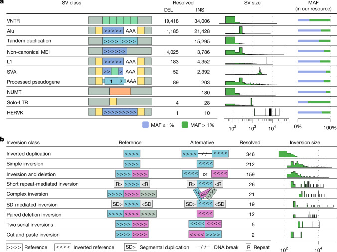
Genomic structural variants (SVs) contribute substantially to genetic diversity and human diseases^1-4, yet remain under-characterized in population-scale cohorts⁵. Here we conducted long-read sequencing⁶ in 1,019 humans to construct an intermediate-coverage resource covering 26 populations from the 1000 Genomes Project. Integrating linear and graph genome-based analyses, we uncover over 100,000 sequence-resolved biallelic SVs and we genotype 300,000 multiallelic variable number of tandem repeats⁷, advancing SV characterization over short-read-based population-scale surveys^3,4. We characterize deletions, duplications, insertions and inversions in distinct populations. Long interspersed nuclear element-1 (L1) and SINE-VNTR-Alu (SVA) retrotransposition activities mediate the transduction^8,9 of unique sequence stretches in 5' or 3', depending on source mobile element class and locus. SV breakpoint analyses point to a spectrum of homology-mediated processes contributing to SV formation and recurrent deletion events. Our open-access resource underscores the value of long-read sequencing in advancing SV characterization and enables guiding variant prioritization in patient genomes.

Fig. 1. LRS and SAGA.

a, Breakdown of self-identified geographical ancestries for 1,019 long-read genomes representing 26 geographies (that is, populations) from 5 continental regions. The three-letter codes used are equivalent to those used in the 1kGP phase III and are resolved in Supplementary Table 2. b, ONT sequence coverage per sample, expressed as fold-coverage (left), and N50 read length in base pairs (right). c, Schematic of the SAGA framework for graph-aware discovery and genotyping of SVs using a pangenome graph augmentation approach. Basemap in a from Natural Earth data (https://www.naturalearthdata.com).

Fig. 2. Callset properties and SV landscape in different geographical ancestries.

a, Cumulative number of unique SVs from the SAGA framework when adding individual long-read genomes, from left to right. The rate of SV discovery slows with each new sample added. Colours denote singletons, doubletons, SVs seen with an allele count of more than 2 (polymorphic), as well as major and shared alleles. b, Left, SV length distributions in population-scale 1kGP SV callsets, versus the cumulative count of SV sites, with a comparison of ONT sequencing (ONT; n = 967 samples) with the short-read-based analysis of the 1kGP cohort (Illumina) subsetted to the same (n = 967) samples. Right, the 1kGP ONT callset is outnumbering short-read-based SV calls both for deletions (DEL, upper sections) and insertions (INS, lower sections). SVs previously unresolved by their sequence, using short reads, are depicted by shaded areas. Notably, LRS provides exact MEI lengths, in contrast to the length approximations reported in short-read-based studies (Supplementary Fig. 29). c, SV allele count (x axis) relative to the count of SV sites (y axis), constructed by genotyping the original HPRC graph (HPRC_mg) and the augmented graph (HPRC_mg_44+966) using Giggles. Consistent with the considerably smaller panel size used, HPRC_mg under-represents rare alleles. d,e, Homozygous (HOM) SV count (d) and heterozygous (HET) SV count (e) per sample stratified into self-identified geographies (n = 967; whiskers extend to points that are within 1.5 × interquartile range from the upper or the lower quartiles). f, Impact of SVs on distinct genomic features. SVs affecting sequences of genes occur at lower MAF compared with non-coding regions. g, Frequency polygons of SV Fst values per continental population (histograms stratifying Fst for bi- and multiallelic are in Supplementary Fig. 28). h, Deletion (DEL) and duplication (DUP) in the intragenic space of two medically relevant genes exhibiting differentiation in AFR and EAS samples, respectively. AC, allele count; AF, allele frequency; CDS, coding sequence; NC, non-coding; UTR, untranslated region.

Fig. 3. Prevalence of distinct SV classes in our SAGA-based data resource.

a, VNTRs (here shown as identified with the SAGA framework), duplications and insertions, as classified by SVAN. The SV class is denoted by label and ideogram, and the number of resolved class members is given for insertions (INS; insertion relative to the reference) and deletions (DEL; deletion relative to reference), in addition to size distribution and percentage of low- and high-frequency alleles. Repeat units for VNTRs and internal VNTR sequence for SVA insertions are depicted using green boxes. TSDs flanking retrotransposition insertion events and LTRs flanking HERVK are represented as yellow boxes. Numbers for interspersed and complex duplications are shown in Supplementary Table 17. Alu, L1 and SVA refer to canonical retrotransposition events. b, Inversion classes identified (twin priming events excluded from this display). For each class, the reference structure is contrasted with the alternative allele, the number of resolved inversions is shown and the inversion size distribution is shown (in bp).

Fig. 4. Polymorphic landscape of L1 and SVA transductions.

a,b, Contribution relative to the total number of transductions (5′, 3′ and orphan) for the 20 most active L1 (a) and SVA (b) progenitors. Source elements are annotated by their presence/absence in the reference, orientation and subfamily. Source element novelty, hot activity status and previously reported activity estimates are based on in vitro assays and transduction tracing (Methods) and are shown as heat maps. Transduction 5′ and 3′ bias was assessed using a two-sided exact binomial test followed by multiple testing correction with Benjamini–Hochberg. Xp22.2 (P_adj = 0.04) and 8q21.11 (P_adj = 3.9 × 10⁻¹⁵) source L1s exhibit a significant 3′ and 5′ bias, respectively. All significant SVAs are 3′ biased, namely 12q24.23 (P_adj = 0.01), 6p12.1 (P_adj = 0.02), 2q33.1-3 (P_adj = 0.02) and 14q11.2-2 (P_adj = 0.04). Adjusted P values for significantly biased loci are represented adjacent to each bar as follows: *P_adj < 0.05; **P_adj < 0.005. c, Circos plot showing the integration positions for the 22 instances of 5′ transductions mediated by the 8q21.11 element. d, Alignment of inserts containing 5′ transductions at the source L1 region, including a single somatic transduction event reported in ref.  in the brain. Inserts are coloured according to whether they align in forward (black) or reverse (blue). Splicing between the full-length L1 and an upstream exon leading to 5′ transductions, highlighted in yellow. e, Magnification showing that the 5′ transductions initiate at a strong promoter located upstream, followed by canonical splicing between the first and second exon of ENSG00000253784, in addition to a second acceptor splice site within the L1 body. Transcription initiation is supported by an annotated transcription start site (hg_93584.1) and CAGE read counts.

Fig. 5. Breakpoint homology landscape and deletion recurrence.

a, Approach for SV breakpoint junction analysis, in the case of primary insertions (INS) achieved by implanting SV sequences into CHM13 (denoted REF). DEL, primary deletion. b, SV length versus homology length (DELs depicted with negative length; INS with positive length). Marginal plots show the size-binned fraction of SV classes perpendicular to both axes, depicting DEL and INS at the left and right, respectively. SVs flanked by repeats are shown in different shades of red (mobile element) and black (SD). SVs exhibiting less than or equal to 15 bp of microhomology or blunt-ended breakpoints are in dark grey. Further colouring denotes: duplications (shades of blue), mobile elements (shades of yellow) and VNTRs (cyan). SVs not classified are in light grey. For visualization purposes, scales of scatter plot axes in a and x axes in b are linear up to 50 bp (representing microhomology) and logarithmic afterwards (representing homology); this split is denoted by the dashed line. c, SV and homology length distribution for distinct SV classes. d, Homology length trend lines for INS and DEL classes combined. e,f, Schematic view showing two repeat-mediated DELs, an Alu-mediated DEL (e) and an SD-mediated DEL (f). g, An 806-bp DEL at 12p13.3 mediated by an AluSx–AluY pair with evidence for recurrence. For visualization purposes, a consensus haplotype in a 20-kb window centred around the DEL is represented for each cluster. Clusters 1–4 were obtained from SNP-based clustering of the haplotypes in a 100-kb window centred around the DEL. Pie charts represent continental ancestries. Squares are used to represent an allele frequency of 0 (yellow) or 1 (cyan) within a cluster, whereas triangles represent allele frequency values in between. A haplotype from HG02546, grouping with cluster 4, is shown as an outlier. Red bars: SNPs indicating deletion recurrence. NHEJ, non-homologous end-joining.

Extended Data Fig. 1. From pseudo haplotypes to generating an augmented graph.

Variant calls within centromere regions are removed and centromere regions are masked by ‘Ns’ in the reference genome. Then, sets of non-overlapping variants are grouped and inserted into the reference genome to obtain “pseudo-haplotypes”. Finally, pseudo-haplotypes are added as new sequences, thereby augmenting the graph, using the minigraph tool.

Extended Data Fig. 2. Evaluation of true positive (TP), false positive (FP) and false negative (FN) SV calls.

a) SV size compared to recently generated multi-platform whole genome assemblies on 16 overlapping samples, for the Giggles genotyped callset, b) SV minor allele frequency (MAF) compared to these whole genome assemblies on 16 overlapping samples, for the Giggles genotyped call set, c) SV size compared to these whole genome assemblies on 16 overlapping samples for the final VCF, which was further filtered for high-quality genotypes emitted by Giggles (Methods) and d) SV MAF compared to these whole genome assemblies, on 16 overlapping samples for the final VCF that was further filtered for high-quality genotypes emitted by Giggles (Methods). DEL, deletion; INS, insertions.

Extended Data Fig. 3. Quality assessment and population characteristics.

a) Quality of the genotypes by Giggles on the HPRC_mg_44 + 966 graph after filtering. Genotyping quality is shown here using a Hardy-Weinberg Equilibrium (HWE) plot given with the allele frequency of the genotyped allele and the percentage of samples heterozygous for that allele (using only the 908 unrelated samples from our dataset). b) SV allele sharing across continental populations. Grey: shared by at least two (and less then all) continental groups. Black: shared by all continental groups. Deletions (top left), insertions (top right), all biallelic SVs (bottom left), all multiallelic (SVs). c) Linkage disequilibrium (LD) of all SVs (MAF > = 1%) with nearby single nucleotide polymorphisms (SNPs). d) As c) with SVs restricted to Genome in a Bottle high-confident regions of the CHM13 genome (2.3 Gbp, 74.2%). e) SV-based admixing spectrum using five reference populations. f) Principal component analysis using all SVs. g) Relation between Variant Allele Count and the Number of Variant Sites with that allele count in the logarithmic space for the SV genotypes on the HPRC_mg_44 + 966 graph, annotated by SVAN. Duplications (DUP), Mobile element insertions and deletions (MEI (non-reference) and MEI (reference), respectively), Nuclear mitochondrial DNA integration (NUMT), processed pseudogene integration (PSD). h) Relationship between the Inversion Allele Count (AC) and the Number of Variant Sites with that allele count shown in log-space for the GeONTIpe based inversion genotypes. The majority of inversions are rare, with most exhibiting an AC < 10. A small subset of inversions is observed more frequently across populations, with 37 inversions exceeding an AC of 1,000, potentially corresponding to reference genome inversions.

Extended Data Fig. 4. VNTR genotyping using vamos.

a-c) Density plots comparing the range difference of repeat unit (RU) counts for different percentile ranges for VNTRs genotyped from our resource (“ONT”) and from multi-platform whole genome assemblies (“HGSVC”), using vamos (plotted range is restricted to data points with x < 100 and y < 100 for visualisation purposes). Plots show guide lines for y = x +/− c with c = 5, 20, 50 for visualizing ranges as shown in the legend below (a-c). Higher c values indicate more extreme cases where one dataset reports higher RU ranges compared to the other (Note S5 and Table S31). d-e) Distribution of the base pair lengths and the count of RUs in the VNTR alleles genotyped by vamos on the ONT data and on the HGSVC assemblies. We depict the distribution of two VNTR loci found in the genes ABCA7 (chr19:1,012,105-1,014,401) in (d) and PLIN4 (chr19:4,494,323-4,497,243) in (e), which have been associated with late-onset human disease^,. For the ABCA7 VNTR locus, alleles of a length greater than 5,720 bp (denoted through a dashed vertical line in (d)) are associated with late-onset disease, whereas for the PLIN4 VNTR locus, alleles with repeat count of 40 (denoted as a dashed vertical line in (e)) are disease-associated. We identify a 43 RU count VNTR allele for the PLIN4 locus in sample NA20127 (outlier denoted with an arrow), with this RU count confirmed using manual inspection (Fig. S62).

Extended Data Fig. 5. Sequence features for polymorphic MEIs annotated using SVAN.

a) At the top we depict a schematic representation of all possible sequence features for canonical L1 insertion conformations, shown as colored boxes. Features include poly-A tails (A(n)) and transductions (TD). Conformations are grouped based on their likely mechanism of origin: target-primed reverse transcription (TPRT) and twin priming (TP). At the bottom left, frequencies of each canonical L1 insertion conformation, where each conformation is defined by a unique combination of the sequence features shown in the schematic. Insertions with configurations inconsistent with TPRT or TP—such as those lacking poly-A tails or containing multiple internal breakpoints—are categorized as non-canonical. At the bottom right, for each L1 insertion conformation, box plots show length distributions of the full insertions and their individual sequence features. Box plots and data points are colored according to the inferred insertion mechanism. b) Stacked dot plots showing alignments of twin priming insertions containing deletions (top) and duplications (bottom) at internal inversion breakpoints. Alignments are colored by orientation, with magenta indicating the inverted L1 sequence. c) Schematic representation of sequence features observed in SVA insertions, along with frequencies of distinct SVA insertion conformations and corresponding length distributions of individual SVA features, shown using the same conventions as for L1 insertions. d, e) Insertion conformations (following the L1 sequence feature colour codes) and length distributions for Alu and processed pseudogene (PSD) insertions.

Extended Data Fig. 6. Polymorphic Human Endogenous Retrovirus Type K (HERV-K) insertions annotated using SVAN.

a, c) Length distributions of HERV-K and solo long terminal repeat (solo-LTR) insertions. b, d) Number of instance specific repetitive DNA element classes overlap the breakpoints for HERV-K and solo-LTR insertions. e) Alignments of HERV-K (top) and solo-LTR (bottom) insertions to the HERV-K113 provirus reference, visualized using the Integrative Genomics Viewer (IGV). Insertion coordinates relative to the CHM13 reference genome, and cytoband identifiers from previously reported insertions. A schematic in the bottom right illustrates the two possible configurations for a full-length HERV-K insertion, with or without an LTR-flanking repeat present in the reference genome.

Extended Data Fig. 7. SV breakpoint homology and microhomology landscape separated by SV annotation.

For all SVs, homology and microhomology was determined. SVs were annotated using the SVAN pipeline as well as by leveraging flanking repeat elements and/or homologous sequence stretches. SVs were grouped into a) repeat-mediated SVs, b) segmental duplication (SD)-mediated SVs, c) duplications (DUP), d) mobile elements (MEI), e) VNTRs, f) not-classified (NA) or NHEJ-mediated SVs. The central scatter plot shows SV length versus (micro)homology length, for each group. Marginal histograms show the distribution of SV length (top) and homology length for deletions (left) and insertions (right). The axes are linear from 0 to 50 bp and log-scale afterwards, which is denoted by a dashed line. To highlight the distribution of rare SV classes, the stacking order in the marginal histograms proceeds from rare (bottom) to common classes (top). Colors correspond to those used in Fig. 5.

Extended Data Fig. 8. Inferred recurrent deletion at 12p13.3.

An inferred recurrent 806 bp deletion at 12p13.3 mediated by an AluSx-AluY pair. The figure shows the variation of haplotypes in a 100 kb window centered around the deletion and the relationship between haplotypes with (red) and without the deletion (grey). Dendrograms of haplotypes are plotted using a centroid hierarchical clustering method. Green dashed lines represent the separation of four haplotype groups shown in Fig. 5g. In each haplotype, reference and alternative alleles are shown in blue and orange, respectively. SNPs within 20 kb around the deletion showing evidence of deletion recurrence are marked by triangles at the top. Two predicted independent occurrences of the deletion event are marked as *1 and *2. The deletion genotypes of the samples involved in these events have been verified by manual inspection of the aligned sequencing reads (Fig. S59).

Extended Data Fig. 9. Patient Genome Analysis.

a) Comparison between SV callsets from ‘rare disease patient A’ generated by PAV and Sniffles, the phased VCF panel of HPRC_mg_44 + 966 and the HGSVC assembly-based SV callset, showing 160 SVs exclusive to the patient genome. b) Allele frequency distributions (log-scale) shown for SV alleles from our study matching those from rare disease patient A, for SVs found both in SAGA and HGSVC (top) and SVs found only in SAGA (bottom). c) Comparison of the number of SVs reported (1) by the pbsv caller (Note S9), (2) by DELLY using default settings, and (3) by DELLY when graph-based filtering is utilised. The median number of SVs detected in 31 rare disease patient genomes are indicated alongside the data points. The comparably high SV count in one patient sample (P1-D11; light orange) is likely attributable to population ancestry. d) An upset plot indicating the number of pathogenic SVs found by DELLY, along with the number of pathogenic SVs retained in graph-based filtering mode (‘delly-pg’). e-f) Integrative Genomics Viewer (IGV) views of the 2 validated pathogenic SVs filtered in pangenome mode. e) A ~ 140 bp insertion in an STR in FMR1 called by DELLY (second row), but not retained in the DELLY-pangenome mode (third row). The length of this multiallelic STR varies in the population, with insert sizes beyond ~450 bp driving the fragile X syndrome. f) A ~ 47 kbp deletion encompassing two regulatory conserved non-coding elements (CNEs) of SHOX is called by DELLY (second row), but not retained in DELLY-pangenome (third row). Variants in the SHOX CNEs exhibit recurrence and incomplete penetrance, consistent with the occasional presence of this SV in the general population (Note S9).

Extended Data Fig. 10. Targeted haplotyping accuracy based on Locityper.

Haplotyping accuracy, here explored in complex loci of the genome across 270 medically relevant loci, is calculated as sequence similarity between two predicted locus haplotypes and actual locus haplotypes, extracted from the whole genome assemblies for 1 sample from the HPRC and 8 samples from a recent multi-platform whole genome assembly study by the Human Genome Structural Variation Consortium (HGSVC). a) Comparison of haplotyping accuracy for high-coverage short-read and intermediate-coverage ONT based haplotypes, inferred using Locityper. b) Improvement in haplotyping accuracy (Locityper accuracy on ONT data minus accuracy on short-read data) across 270 loci. The inset shows 20 genes with the highest improvement in haplotyping accuracy.

References

1. Spielmann, M., Lupiáñez, D. G. & Mundlos, S. Structural variation in the 3D genome. Nat. Rev. Genet.19, 453–467 (2018). - PubMed
1. Weischenfeldt, J., Symmons, O., Spitz, F. & Korbel, J. O. Phenotypic impact of genomic structural variation: insights from and for human disease. Nat. Rev. Genet.14, 125–138 (2013). - PubMed
1. Byrska-Bishop, M. et al. High coverage whole genome sequencing of the expanded 1000 Genomes Project cohort including 602 trios. Cell185, 3426–3440.e19 (2022). - PMC - PubMed
1. Sudmant, P. H. et al. An integrated map of structural variation in 2,504 human genomes. Nature526, 75–81 (2015). - PMC - PubMed
1. Rausch, T., Marschall, T. & Korbel, J. O. The impact of long-read sequencing on human population-scale genomics. Genome Res.35, 593–598 (2025). - PMC - PubMed
LinkOut - more resources