AI-driven multi-omics modeling of myalgic encephalomyelitis/chronic fatigue syndrome

Abstract

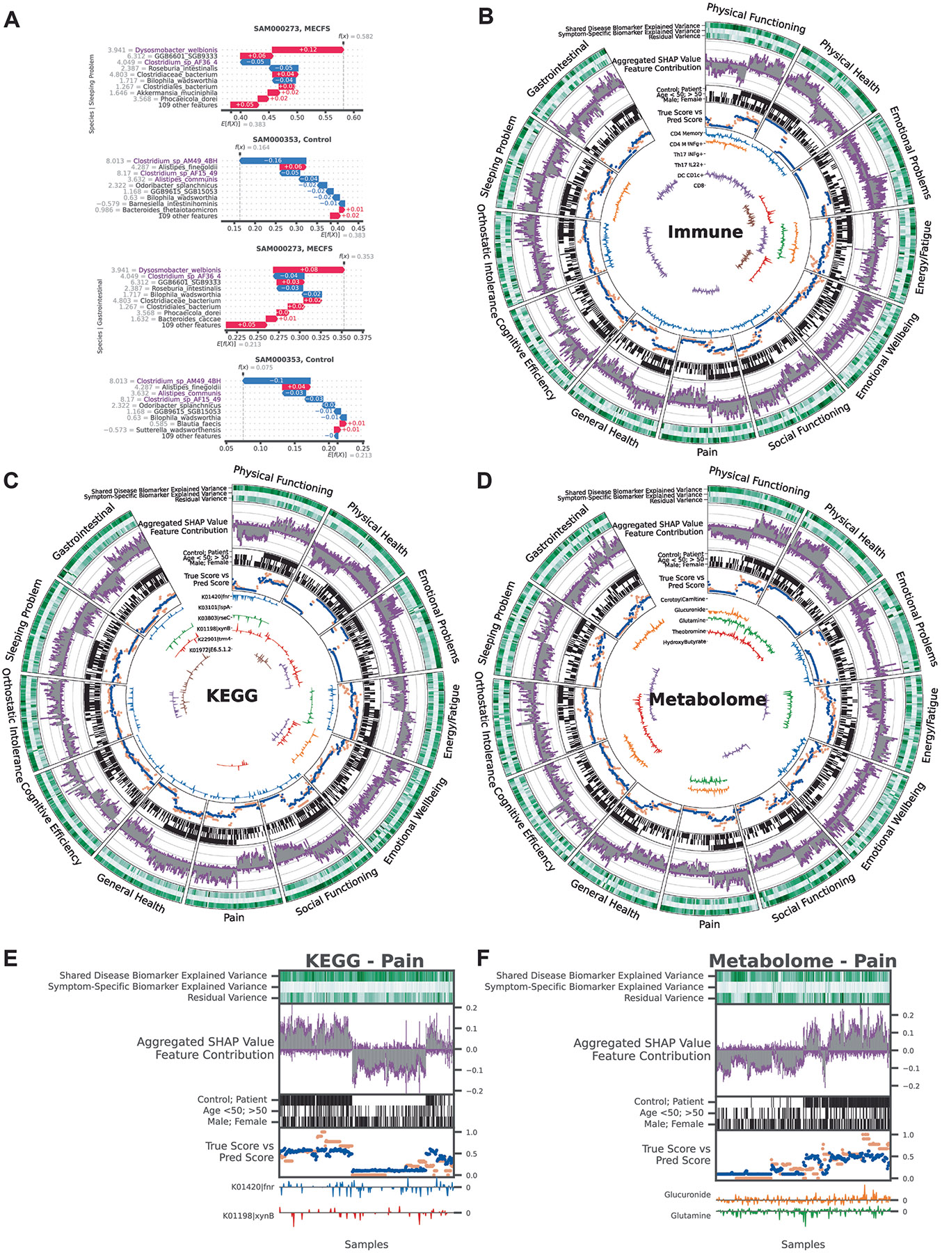
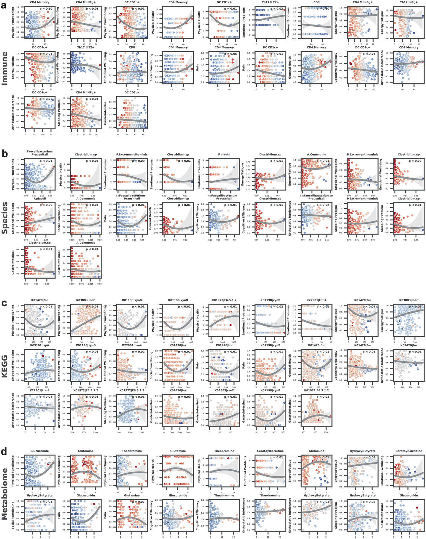
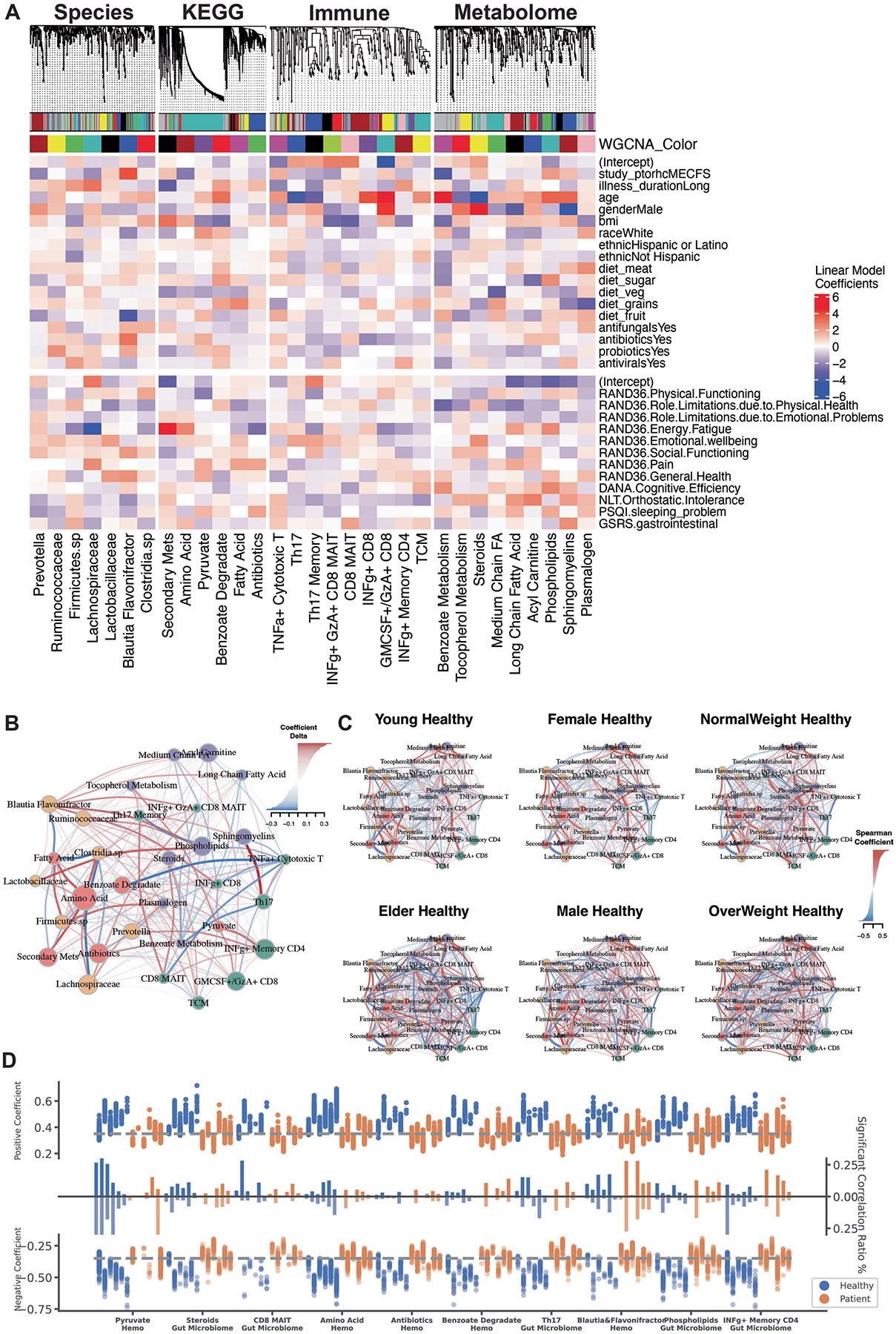
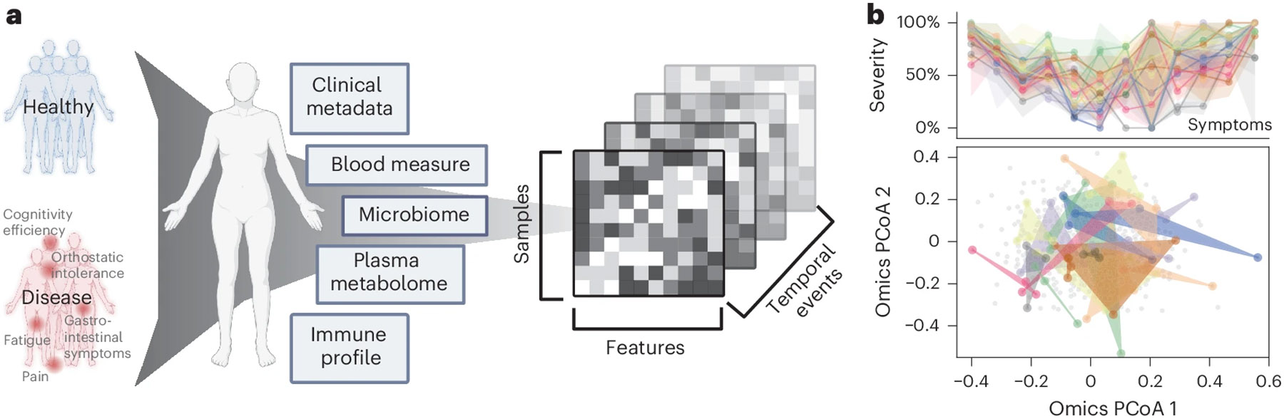
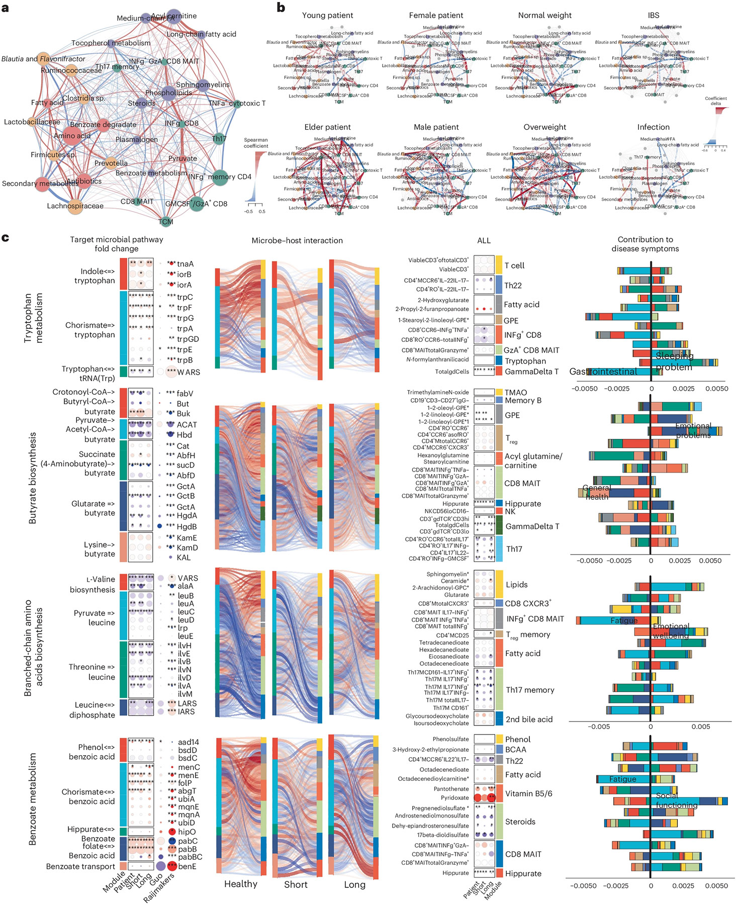
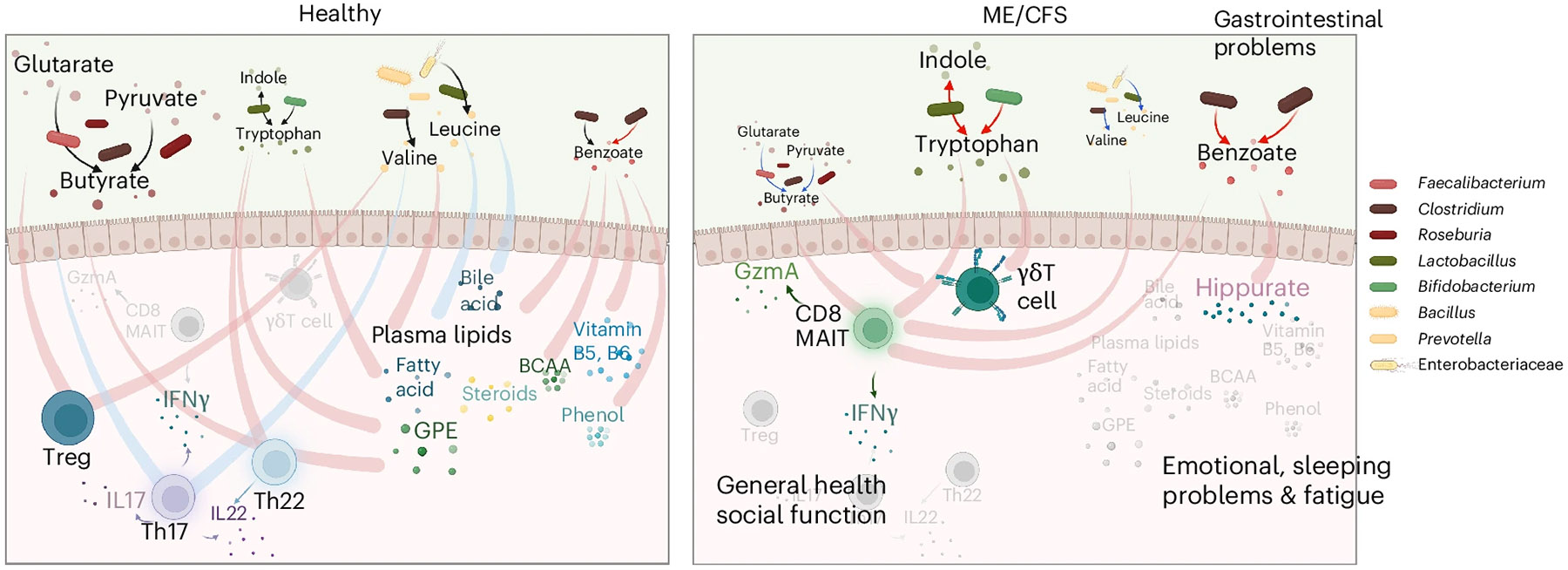
Myalgic encephalomyelitis/chronic fatigue syndrome (ME/CFS) is a chronic illness with a multifactorial etiology and heterogeneous symptomatology, posing major challenges for diagnosis and treatment. Here we present BioMapAI, a supervised deep neural network trained on a 4-year, longitudinal, multi-omics dataset from 249 participants, which integrates gut metagenomics, plasma metabolomics, immune cell profiling, blood laboratory data and detailed clinical symptoms. By simultaneously modeling these diverse data types to predict clinical severity, BioMapAI identifies disease- and symptom-specific biomarkers and classifies ME/CFS in both held-out and independent external cohorts. Using an explainable AI approach, we construct a unique connectivity map spanning the microbiome, immune system and plasma metabolome in health and ME/CFS adjusted for age, gender and additional clinical factors. This map uncovers altered associations between microbial metabolism (for example, short-chain fatty acids, branched-chain amino acids, tryptophan, benzoate), plasma lipids and bile acids, and heightened inflammatory responses in mucosal and inflammatory T cell subsets (MAIT, γδT) secreting IFN-γ and GzA. Overall, BioMapAI provides unprecedented systems-level insights into ME/CFS, refining existing hypotheses and hypothesizing unique mechanisms-specifically, how multi-omics dynamics are associated to the disease's heterogeneous symptoms.

Extended Data Fig. 1 ∣. Data Pairedness Overview and Heterogeneity in Healthy and Patients.

a, Cohort Composition and Data Collection. Over four years, 515 time points were collected: baseline year from all 249 donors (Healthy N=96, ME/CFS N=153); second year from 168 individuals (Healthy N=58, ME/CFS N=110); third year from 94 individuals (Healthy N=13, ME/CFS N=81); fourth year from N=4 ME/CFS patients. Clinical metadata and blood measures were collected at all 515 points. Immune profiles from PBMCs were recorded at 489 points, microbiome data from stool samples at 479 points, and plasma metabolome data at 414 points. A total of 1,471 biosamples were collected. b-c, Heterogeneity of b, Healthy Controls and c, All Patients in Symptom Severity and omics Profiles. Supplemental information for Fig. 1b, which shows examples from 20 patients. Variability in symptom severity (top) and omics profiles (bottom) for all healthy controls and all patients with 3-4 time points. The top x-axis numbers represent 12 symptoms, arranged in the same order as Extended Data Fig. 1f, g (left to right, top to bottom). d, Distribution of 12 Clinical Symptoms in ME/CFS and Control. Density plots compare the distributions of 12 clinical scores between control (blue) and ME/CFS patients (orange) with the x-axis represents the values of symptom severity (scaled from 0%, no symptom, to 100%, most severe) and the y-axis represents the frequency (count) of data points. e, Principal Coordinates Analysis (PCoA) of each ‘Omics. PCoA based on Bray-Curtis distance. Control samples (blue) and ME/CFS patients (red) show distinct clustering. Here, except for the clinical scores, controls are indistinguishable from patients, highlighting the difficulty of building classification models. f-g, Symptom Progression Over Time in f, Healthy vs. g, ME/CFS Patients. Symptom progression for each individual (represented by different colors) is shown using line plots of symptom severity (y-axis) over time points (years 1–4). Compared to healthy controls, ME/CFS patients exhibit higher severity, greater heterogeneity, and inconsistent or nonlinear progression (indicated by substantial variation over time without a consistent pattern) in clinical symptoms. Related to: Figs. 1-2.

Extended Data Fig. 2 ∣. BioMapAI’s Performance at Clinical Score Reconstruction and Disease Classification.

a, Density map of True vs. Predicted Clinical Scores. Supplemental information for Fig. 2b, which shows three examples. Here, the full set of 12 clinical scores compares the true score, $y$ (Column 1), against BioMapAI’s predictions generated from different omics profiles – ${\widehat{y}}_{immune}$, ${\widehat{y}}_{species}$, ${\widehat{y}}_{KEGG}$, ${\widehat{y}}_{metabolome}$, ${\widehat{y}}_{quest}$, ${\widehat{y}}_{omics}$ (Columns 2–7). b, Scatter Plot of True vs. Predicted Clinical Scores. Scatter plots display the relationship between true clinical scores (x-axis) and predicted clinical scores (y-axis) for six different models: Omics, Immune, Species, KEGG, Metabolome, and Quest Labs. Each plot demonstrates the clinical score prediction accuracy for each model. c, ROC Curve for Disease Classification with Original Clinical Scores. The Receiver Operating Characteristic (ROC) curve evaluates the performance of disease classification using the original 12 clinical scores. The mean Area Under the Curve (AUC) is 0.99, indicating high prediction accuracy, which aligns with the clinical diagnosis of ME/CFS based on key symptoms. d, 3D t-SNE Visualization of Hidden Layers. 3D t-SNE plots show how BioMapAI progressively distinguishes disease from control across hidden layers for five trained ‘omics models: Immune, KEGG, Species, Metabolome, and Quest Labs. Each plot uses the first three principal components to show the spatial distribution of control samples (blue) and ME/CFS patients (red). The progression from the input layer (mixed groups) to Hidden Layer 3 (fully separated groups) illustrates how BioMapAI progressively learns to separate ME/CFS from healthy controls. Related to: Fig. 2.

Extended Data Fig. 3 ∣. Disease-Specific Biomarkers - Top 10 Biomarkers Shared across Clinical Symptoms and Multiple Models.

Through the top 30 high-ranking features for each score, we discovered that the most critical features for all 12 symptoms were largely shared and consistently validated across ML and DL models, particularly the foremost 10. Here, this multi-panel figure presents the top 10 most significant features identified by BioMapAI across five omics profiles, highlighting their importance in predicting clinical symptoms and diagnostic outcomes across BioMapAI, DNN, and GBDT models, along with their data prevalence. Each vertical section represents one omics profile, with columns of biomarkers ordered by average feature importance from right to left. From top to bottom: 1. Heatmap of SHAP Values from BioMapAI. This heatmap shows averaged SHAP values with the 12 scores on the rows and the top 10 features in the columns. Darker colors indicate a stronger impact on the model’s output; Consistency among the top 5 features suggests they are shared disease biomarkers crucial for all clinical symptoms; 2. Swarm Plot of SHAP Values from DNN. This plot represents the distribution of feature contributions from DNN, which is structurally similar to BioMapAI but omits the third hidden layer ($Z^3$). SHAP values are plotted vertically, ranging from negative to positive, showing each feature’s influence on prediction outcomes. Points represent individual samples, with color gradients denoting actual feature values. For instance, Dysosmobacteria welbionis, identified as the most critical species, shows that greater species relative abundance correlates with a higher likelihood of disease prediction; 3. Bar Graphs of Feature Importance in GBDT. GBDT is another machine learning model used for comparison. Each bar’s height indicates a feature’s significance within the GBDT model, providing another perspective on the predictive relevance of each biomarker; 4. Heatmap of Normalized Raw Abundance Data. This heatmap compares biomarker prevalence between healthy and disease states, with colors representing z-scored abundance values, highlighting biomarker differences between groups. Supporting Materials: Extended Data Table 3. Related to: Fig. 3.

Extended Data Fig. 4 ∣. Symptom-Specific Biomarkers - Immune, KEGG and Metabolome Models.

By linking omics profiles to clinical symptoms, BioMapAI identified unique symptom-specific biomarkers in addition to disease-specific biomarkers (Extended Data Fig. 3). Each omics has a circularized diagram (Fig. 3a, Extended Data Fig. 4b-d) to display how BioMapAI use this omics profile to predict 12 clinical symptoms and to discuss the contribution of disease- and symptom-specific biomarkers. Detailed correlation between symptom-specific biomarkers and their corresponding symptoms is in Extended Data Fig. 5. a, Examples of Sleeping Problem-Specific Species’ and Gastrointestinal-Specific Species’ Contributions. Supplemental information for Fig. 3d, which shows the contribution of pain-specific species. b-d, Circularized Diagram for Immune, KEGG and Metabolome Models. Supplemental information for Fig. 3a, which shows the species model. e-f, Zoomed Segment for Pain in KEGG and Metabolome Model. Supplemental information for Fig. 3b, which shows the zoomed segment for pain in the species and immune models. *Note, the reported biomarkers were calculated using the entire dataset and were not validated on held-out data. Abbreviations and Supporting Materials: Extended Data Fig. 5. Related to: Fig. 3.

Extended Data Fig. 5 ∣. Symptom-Specific Biomarkers - Different Correlation Patterns of Biomarkers to Symptom.

Supplemental information for Fig. 3c, which shows six pain biomarkers from multiple models. Here for each omics (a-d, Immune, Species, KEGG, Metabolome), we plotted the correlation of symptom-specific biomarkers (x-axis) to its related symptom (y-axis), colored by SHAP value (contribution to the symptom). P value by two-sided spearman correlation, FDR adjusted (Detailed statistics in Supplementary Table 5). Abbreviations: CD4, Cluster of Differentiation 4; CD8, Cluster of Differentiation 8; IFNg, Interferon Gamma; DC, Dendritic Cells; MAIT, Mucosal-Associated Invariant T; Th17, T helper 17 cells; CD4+ TCM, CD4+ Central Memory T cells; DC CD1c+ mBtp+, Dendritic Cells expressing CD1c+ and myelin basic protein; DC CD1c+ mHsp, Dendritic Cells expressing CD1c+ and heat shock protein; CD4+ TEM, CD4+ Effector Memory T cells; CD4+ Th17 rfx4+, CD4+ T helper 17 cells expressing RFX4; F. prausnitzii, Faecalibacterium prausnitzii; A. communis, Akkermansia communis; NAD, Nicotinamide Adenine Dinucleotide. Related to: Fig. 3.

Extended Data Fig. 6 ∣. omics WGCNA Modules and Host-Microbiome Network.

a, Correlation of WGCNA Modules with Clinical Metadata. Weighted Gene Co-expression Network Analysis (WGCNA) was used to identify co-expression modules for each omics layer: species, KEGG, immune, and metabolome. The top dendrograms show hierarchical clustering of ‘omics features, with modules identified. The bottom heatmap shows the relationship of module eigengenes (colored as per dendrogram) with clinical metadata – including demographic information and environmental factors - and 12 clinical scores. General linear models were used to determine the primary clinical drivers for each module, with the color gradient representing the coefficients (red = positive, blue = negative). Microbial modules were influenced by disease presence and energy-fatigue levels, while metabolome and immune modules correlated with age and gender. b-c, Microbiome-Immune-Metabolome Network in b, Patient and c, Healthy Subgroups. Supplemental information for Fig. 4a (Healthy Network) and 4b (Patient Subgroups). Figure 4a is the healthy network; here, Extended Data Fig. 6b presented the shifted correlations in all patients. Figure 4b represented the network in patient subgroups; here, Extended Data Fig. 6c is the corresponding healthy counterpart, for example, female patients were compared with female controls to exclude gender influences. d, Differences in Host-Microbiome Correlations between Healthy and Patient Subgroups. Selected host–microbiome module pairs are grouped on the x-axis (for example, pyruvate to blood modules, steroids to gut microbiome). Significant positive and negative correlations (top and bottom y-axis) of module members pairs are shown as dots for each subgroup (blue = healthy, orange = patient) (Spearman, adjusted p < 0.05), from left to right: Young, Elder, Female, Male, NormalWeight, OverWeight Healthy and Young, Elder, Female, Male, NormalWeight, OverWeight Patient. The middle bars represent the total count of associations. This panel highlights the shifts in host–microbiome networks from health to disease, for example, in patients, the loss of pyruvate to host blood modules correlation and the increase of INFg+ CD4 memory correlation with gut microbiome. Related to: Fig. 4.

Fig. 1 ∣. Cohort summary and heterogeneity of ME/CFS.

a, Cohort design and omics profiling. 96 healthy donors and 153 patients with ME/CFS were followed over 3 to 4 years with yearly sampling. Clinical metadata including lifestyle and dietary surveys, blood clinical laboratory measures ($n=503$), gut microbiome ($n=479$), plasma metabolome ($n=414$) and immune profiles ($n=489$) were collected (Supplementary Table 1 and Extended Data Fig. 1a). Created in BioRender. Xiong, R. (2025) https://BioRender.com/adqusn8. b, Heterogeneity and nonlinear progression of ME/CFS in symptom severity and omics profiles. This section highlights variability in symptom severity (top) and omics profiles (bottom) for 20 representative patients with ME/CFS over three to four time points. Top: symptom severity is shown for 12 major clinical symptoms ($x$ axis, with each column representing one symptom) against severity scores (scaled from 0% (no symptom) to 100% (most severe), $y$ axis) for each patient (each represented by a distinct color). Lines indicate average severity, and shaded areas represent the severity range across time points (controls shown in Extended Data Fig. 1b). For ME/CFS symptomatology, b (top) highlights substantial heterogeneity over time, as shown by the widespread shaded areas. Extended Data Fig. 1f,g further confirms the absence of consistent temporal patterns, with symptom severity fluctuating considerably over time. Notably, among the 12 symptoms, trends differed: fatigue (symptom 1) remains consistently severe over years, whereas emotional dysregulation (symptom 8) exhibits notable variability and instability over time (Extended Data Fig. 1g). Bottom: PCoA of integrated omics data. The background gray dots represent the entire cohort, defining the overall range of variation in the PCoA space. Colored dots highlight omics-level heterogeneity, with each set of same-colored dots corresponding to an individual’s different time points. The spread and overlap of the colored space reflect the diversity in omics signatures of patients versus the more consistent pattern typical of controls (Extended Data Fig. 1c).

Fig. 2 ∣. BioMapAI’s model structure and performance.

a, BioMapAI’s structure. BioMapAI is a fully connected DNN composed of an input layer ($X$), a normalization layer, three sequential hidden layers ($Z^1$, $Z^2$, $Z^3$), and one output layer ($Y$). Hidden layer $Z^1$ (64 nodes) and hidden layer $Z^2$ (32 nodes) feature a dropout ratio of 50% to prevent overfitting. Hidden layer 3 has 12 parallel sublayers, each with 8 nodes ($Z^3=[z_1^3,z_2^3,\dots ,z_{12}^3]$) to learn 12 objects in the output layer ($Y=[y^1,y^2,\dots ,y^{12}]$) representing key clinical symptoms of ME/CFS. In total, we used six inputs ($X$): five individual omics and one merged omics integrating the most important features. Created in BioRender. Xiong, R. (2025) https://BioRender.com/v9fnv0r. b, True versus predicted clinical scores highlight BioMapAI’s accuracy. Three example density maps (full set, Extended Data Fig. 2a) compare the true score, $y$ (Column 1) against BioMapAI’s predictions generated from different omics. $y$ axis represents the diversity along the $x$ axis for each omics. Color gradient from blue (lower density) to red (higher density) illustrates the occurrence frequency, with dashed lines indicating key statistical percentiles. c, Omics’ strengths in symptom prediction. Each of the 12 axes represents a clinical score output ($Y=[y_1,y_2,\dots ,y_{12}]$), with five colors denoting the omics datasets used for model training. The spread of each color along an axis reflects the 1 – normalized mean square error (MSE) (Supplementary Table 2) between the actual, $y$, and the predicted, $\widehat{y}$, outputs, illustrating the predictive strength or weakness of each omics for specific clinical scores. The radial scale ranges from 0.8 (center) to 1.0 (outer circle), where values closer to the outer edge correspond to lower MSE and better predictions. d, BioMapAI’s performance in healthy versus disease classification (10-fold cross-validation and held-out data). ROC curves show BioMapAI’s performance in disease classification using each omics dataset separately or combined (‘Omics’), with the AUC in parentheses showing prediction accuracy (full report in Supplementary Table 3). The dashed line represents a baseline for comparison. e, Validation of BioMapAI with external cohorts. External cohorts with microbiome data (Guo, Raijmakers) and metabolome data (Germain, Che) were used to test BioMapAI’s model, underscoring its prediction accuracy (detailed classification matrix, Supplementary Table 3).

Fig. 3 ∣. BioMapAI identifies both disease- and symptom-specific biomarkers.

a,b, For symptom-specific biomarkers, circularized diagram of species model (a) with zoomed segment for pain (b). Each circular panel illustrates how the model predicts 12 symptom-specific biomarkers derived from one omics (all data in Extended Data Fig. 4); $x$ axis represents individuals. The reported biomarkers were not validated on held-out data. From top to bottom: 1. variance explained by biomarker categories (gradients of dark green (100%) to white (0%) show variance explained by the model); 2. aggregated SHAP values quantify the contribution of each feature to the model’s predictions (disease-specific biomarkers in gray and symptom-specific in purple); 3. demography and cohort classification (cohort (controls, white versus patients, black); age <50 years (white) versus >50 (black); sex (male, white vs. female, black)); 4. true versus predicted scores show BioMapAI’s predictive performance at the individual sample level (true in blue and model-predicted scores in orange); 5. examples of symptom-specific biomarkers (line graphs show the contribution of select symptom-specific biomarkers to the model across individuals). Peaks above 0 (middle line) indicate positive and below 0 for negative. c, Different correlation patterns of biomarkers to symptoms. For pain (see also Extended Data Fig. 5), correlation analysis of raw abundance ($x$ axis) with pain score ($y$ axis) show monotonic (for example, CD4 memory and DC CD1c⁺ markers), biphasic (microbial and metabolomic markers) or sparse (KEGG genes) contributions. Dots represent an individual color-coded to SHAP value, where the color spectrum indicates negative (blue) to neutral (gray) to positive (red) contributions to pain prediction. Superimposed trend lines with shaded error bands represents the predicted correlation trends. Adjacent bar plots represent the data distribution. P value by two-sided Spearman correlation, FDR adjusted (detailed statistics in Supplementary Table 5). d,e, Examples of pain-specific species (d) and immune (e) biomarkers’ contributions. SHAP waterfall plots illustrate the contribution of individual features to predictive output. The top 10 features are shown here, illustrating the species and the immune model (additional examples in Extended Data Fig. 4a). The contribution of each feature is shown as a step, and the cumulative effect of all the steps provides the final prediction value, $E[f(X)]$.

Fig. 4 ∣. Microbiome-immune-metabolome crosstalk is dysbiotic in ME/CFS.

a,b, Microbiome-immune-metabolome network in healthy (a) and patient (b) subgroups. A baseline network was established with 200+ healthy control samples (a), bifurcating into two segments: the gut microbiome (species in yellow, genetic modules in orange) and blood elements (immune modules in green, metabolome modules in purple). Nodes: modules; size: number of members; colors: omics type; edges: interactions between modules, with Spearman coefficient (adjusted) represented by thickness, transparency and color—positive (red) and negative (blue). Here, key microbial pathways (pyruvate, amino acid and benzoate) interact with immune and metabolome modules in healthy individuals. Specifically, these correlations were disrupted in patient subgroups (b), as a function of gender, age (young <26 years versus older >50 years), BMI (normal <26 versus overweight >26) and health status (individuals with IBS or infections). Correlations significantly shifted from healthy counterparts (Extended Data Fig. 6c) are highlighted with colored nodes and edges indicating increased (red) or decreased (blue) interactions. c, Targeted microbial pathways and host interactions. Four microbial metabolic mechanisms were analyzed to compare control, short- and long-term patients with ME/CFS, and external cohorts for validation (Guo and Raijmakers) along with their associated host immune/metabolome modules. 1. Microbial pathway fold change: key genes were grouped and annotated in subpathways. Circle size: fold change over control; color: increase (red) or decrease (blue), P values (patient versus control, P value by two-sided Wilcoxon, FDR adjusted; detailed statistics in Supplementary Table 8) marked. 2. Microbiome–host interactions: Sankey diagrams visualize interactions between microbial pathways and host immune cells/metabolites. Line thickness and transparency: Spearman coefficient (adjusted); color: red (positive), blue (negative). 3. Immune and metabolites fold change: pathway-correlated immune cells and metabolites are grouped by category. 4. Contribution to disease symptoms: stacked bar plots show accumulated SHAP values (contributions to symptom severity) for each disease symptom (1–12, as in Supplementary Table 1). Colors: microbial subpathways and immune/metabolome categories match module color in fold change maps. $x$ axis: accumulated SHAP values (contributions) from negative to positive, with the most contributed symptoms highlighted. P values: *P < 0.05, **P < 0.01, ***P < 0.001.

Fig. 5 ∣. Overview of dysbiotic host–microbiome interactions in ME/CFS.

This conceptual diagram visualizes the host–microbiome interactions in healthy conditions (left) and its disruption and transition into the disease state in ME/CFS (right). The base icons of the figure remain consistent, whereas gradients and changes in color and size visually represent the progression of the disease. Process of production and processing is represented by lines with arrows, where the color indicates an increase (red) or decrease (blue) in the pathway in disease; lines without arrows indicate correlations, with red representing positive and blue representing negative correlations. In healthy conditions, microbial metabolites support immune regulation, maintaining mucosal integrity and healthy inflammatory responses by positively regulating T_reg and Th22 cell activity, and controlling Th17 activities, including the secretion of IL-17 (purple cells), IL-22 (blue) and IFN-γ. These microbial metabolites also maintain many positive interactions with plasma metabolites like lipids, bile acids, vitamins and phenols. In ME/CFS, there is a significant decrease in beneficial microbes and a disruption in metabolic pathways, marked by a decrease in the butyrate (brown-red dots) and BCAA (yellow) pathways and an increase in tryptophan (green) and benzoate (red) pathways. These changes are linked to gastrointestinal issues. In ME/CFS, the regulatory capacity of the immune system diminishes, leading to the loss of health-associated interactions with Th17, Th22 and T_reg cells, and an increase in inflammatory immune activity. Pathogenic immune cells, including CD8 MAIT and γδT cells, show increased activity, along with the secretion of inflammatory cytokines such as IFN-γ and GzmA, contributing to worsened general health and social functioning. Healthy interactions between gut microbial metabolites and plasma metabolites weaken or even reverse in the disease state. A notable strong connection increased in ME/CFS is benzoate transformation to hippurate, associated with emotional disturbances, sleep issues, and fatigue. Created in BioRender. Xiong, R. (2025) https://BioRender.com/cje1xlx.

References

1. Ruiz-Pablos M, Paiva B, Montero-Mateo R, Garcia N & Zabaleta A. Epstein-Barr virus and the origin of myalgic encephalomyelitis or chronic fatigue syndrome. Front. Immunol 12, 656797 (2021). - PMC - PubMed
1. Su R. et al. The TLR3/IRF1/type III IFN axis facilitates antiviral responses against enterovirus infections in the intestine. mBio 11, e02540–20 (2020). - PMC - PubMed
1. Anderson DE et al. Lack of cross-neutralization by SARS patient sera towards SARS-CoV-2. Emerg Microbes Infect. 9, 900–902 (2020). - PMC - PubMed
1. Cairns R & Hotopf M. A systematic review describing the prognosis of chronic fatigue syndrome. Occup. Med. Oxf. Engl 55, 20–31 (2005).
1. Cortes Rivera M, Mastronardi C, Silva-Aldana CT, Arcos-Burgos M & Lidbury BA Myalgic encephalomyelitis/chronic fatigue syndrome: a comprehensive review. Diagnostics 9, 91 (2019). - PMC - PubMed
MeSH terms
LinkOut - more resources