Representational drift as the consequence of ongoing memory storage

Abstract

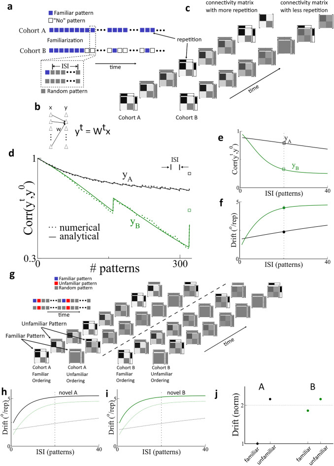
Memory systems with biologically constrained synapses have been the topic of intense theoretical study for over thirty years. Perhaps the most fundamental and far-reaching finding from this work is that the storage of new memories implies the partial erasure of already-stored ones. This overwriting leads to a decorrelation of sensory-driven activity patterns over time, even if the input patterns remain similar. Representational drift (RD) should therefore be an expected and inevitable consequence of ongoing memory storage. We tested this hypothesis by fitting a network model to data from long-term chronic calcium imaging experiments in mouse hippocampus. Synaptic turnover in the model inputs, consistent with the ongoing encoding of new activity patterns, accounted for the observed statistics of RD. This mechanism also provides a parsimonious explanation for the diverse effects of experience on drift found in experiment. Our results suggest that RD should be observed wherever neuronal circuits are involved in a process of ongoing learning or memory storage.

Fig. 1

Ongoing memory storage generates representational drift. (a) Memories are encoded in an ongoing fashion in time. Memory identity is indicated by color. We track and observe the neuronal activity corresponding to one memory in particular (pink square). (b) Synaptic weights undergo plasticity as memories are stored. When pre- and post-synaptic activity is high, synapses may undergo potentiation (large red circle), while depression takes place if one cell fires strongly and the other only weakly (small blue circle). Active presynaptic cells are indicated by a train of action potentials. The postsynaptic cell fires strongly (black) or weakly (grey). Synaptic weights are strong (large circle) or weak (small circle). Note that due to the plasticity from the two intervening memories, the response of the post-synaptic cell to the same pre-synaptic pattern of activity, corresponding to the pink memory, has changed: its firing rate has decreased. (c) The change in post-synaptic activity due to ongoing memory storage manifests itself at the population level as representational drift. Therefore, there is a drop in correlation between the initial pattern of neuronal activity given inputs corresponding to the pink memory and the first repetition . If we assume that ongoing memory storage occurs between every repetition the correlation will continue to decrease. LTP: Long-term potentiation. LTD: Long-term depression.

Fig. 2

A spiking network model with random synaptic turnover reproduces drift dynamics (a) Network architecture and sample raster plot of CA1 pyramidal cells. (b) Heterogeneous response profiles for sample CA1 cells. The color indicates the value of spatial information from c. (c) Histogram of spatial information for all CA1 cells over one session. (d) Synaptic turnover from session to session is modeled by randomly rewiring a fraction of inputs to each CA1 pyramidal cell, independently for EC versus CA3 pathways. (e) Tuning curve (top row) and total input (bottom row) for one example cell over three sessions. The dashed line in the bottom panel indicates the average total input along the track for each session. (f) Place field maps for 200 randomly selected active cells found on session 1 (top) or session 8 (bottom), ordered according to their place field positions. (g) PV correlation of all cells (left), and only place cells (cells significantly spatially tuned in both sessions) (right). The insets show the first four points of the respective curves, where the initial point (within-session correlation) is computed considering odd vs even trials. (h) Distribution of the centroid shift for different number of elapsed sessions (color-coded). Inset: cumulative distribution of the absolute shift. See “Methods” section for model details and parameter values.

Fig. 3

Synaptic turnover is consistent with the ongoing storage of random patterns. (a–c) The synaptic turnover model. (a) Changes in inputs from one session to the next are modeled as a rewiring of synaptic connections. (b) The probability for a connection begin removed or added is given by and respectively, while the rewiring fraction is defined as the sum of the two. (c) Schematic of rewired connections after one time step. (d–f) The Hebbian plasticity model. (d) Changes in inputs from one session to the next are due to the encoding of random, uncorrelated patterns through Hebbian plasticity. (e) Synapses are removed or added through activity-dependent depression and potentiation, which occur with probabilities and respectively. (f) Schematic of plasticity after one time step. (g) The drift observed in experiment in CA1 can be modeled either through synaptic turnover, as in Fig. 2, or, as illustrated here, by assuming the encoding of episodes between sessions through Hebbian learning. (h) The Hebbian process is fit to the synaptic turnover by matching the drop in correlation in input to CA1 cells over sessions. The circles indicate the values of correlation which correspond to the snapshots of activity shown in Fig. 2f, see “Methods” section for details and parameter values.

Fig. 4

Ongoing memory storage is consistent with differential effects of drift on rate and tuning (a) We consider the storage of many memories, indicated here by color, all with spatial and non-spatial features, and one of which (pink) is tracked explicitly. Only changes to synapses which are active in that environment (dashed boxes in cell schematic) will generate observable RD. In the limit of sparse place cell coding the storage of the blue and orange memories readily causes drift in non-spatial inputs, but not in the spatial ones. As a result, RD in non-spatial features is proportional to the total number of memories stored, while RD in spatial tuning is due only to repetitions of the tracked memory. (b) Simulation protocol for which the repetition rate for environment A is twice that of B. In the sparse spatial coding limit the rate correlation depends on total patterns stored (time) while the tuning correlation depends only on repetitions of the tracked pattern (session). (c) Schematic of network model. Tuned and untuned inputs are summed and thresholded to determine the activity of CA1 pyramidal cells. The connectivity undergoes Hebbian plasticity according to the model in Fig. 3. (d) Results of simulations when the sparseness of spatial coding . The drop in tuning correlation is affected both the number of repetitions as well as interference from other memories. (e,f) When spatially tuned inputs already exhibit drift, as has been observed in CA3 place cells, the combined effect of sparseness and drift results in the tuning correlation being dominated by the number of repetitions. See “Methods” section for model details and parameter values.

Fig. 5

Repeated exposure to same input pattern reduces drift (a) Protocol for testing the effect of repetition rate on drift. Two cohorts are repeatedly presented a pattern (blue squares) during a familiarization period. After this time cohort A is presented the familiar pattern every session while B is presented the familiar pattern every eight sessions. Crucially, we assume that a number of additional patterns, uncorrelated with the familiar one are encoded between sessions (inter-session interval, ISI) (grey squares). (b) Schematic of the model. Here there is only one input layer, and there is no spatial selectivity. The synaptic connectivity matrix W is updated according to the same Hebbian rule used in Figs. 3 and 4. (c) Illustration of the effect of repetition rate on network connectivity. Repetition boosts network structure correlated with the familiar pattern, thereby reducing drift. (d) Output correlation for familiarized pattern with a total of 16 repetitions for cohort A and , while the repetition rate for B was 8 times less. Dotted lines are from simulation of the network model with Hebbian plasticity while solid lines are the solution of the corresponding Markov process. (e,f) Output correlation and drift rate as a function of the ISI, i.e. the number of random patterns encoded between “sessions”. The vertical line indicates the value of ISI used in (d,g) Illustration of encoding of familiar and unfamiliar patterns. Because the repetition rate is the same for the unfamiliar pattern for both cohorts, the resultant drift is also the same. (h,i) Drift rates for the unfamiliar patterns. (j) Drift rates normalized by the familiar case for cohort A. Parameters: , , . For the familiar cases the tracked pattern was encoded times at time zero, whereas for the novel cases . See “Methods” section for model details.

Fig. 6

How familiarity and input stability modulate RD. (a) We model familiarity by presenting a given pattern to the network k times before time , i.e. is a novel pattern. Here , and . (b) Same as in (a) but with . (c) Correlation after a total of 320 patterns, with either 16 or 2 repetitions, for low and high learning rates. (d) The input patterns driving the observed activity may themselves undergo RD, which we parameterize with s. Here indicates completely stable inputs over time while indicates that the input vectors are completely uncorrelated from repetition to repetition. (E) When inputs are stable, increased repetition rate decreases RD , while this need not be the case when inputs themselves drift . (F) The repetition rate can reduce RD (black lines), increase RD (green line) or even leave it largely unchanged (orange line).

References

1. Hebb, D. The Organization of Behavior (John Wiley and Sons, 1949).
1. Hopfield, J. Neural networks and physical systems with emergent collective computational abilities. PNAS79, 2554–2558 (1982). - PMC - PubMed
1. Amit, D., Gutfreund, H. & Sompolinsky, H. Spin-glass models of neural networks. Phys. Rev. A32, 1007–1018 (1985). - PubMed
1. Tsodyks, M. & Feigel’man, M. The enhanced storage capacity in neural networks with low activity level. Europhys. Lett.6, 101–105 (1988).
1. Amit, D. & Fusi, S. Constraints on linearning in dynamics synapses. Netw. Comput. Neural Syst.3, 443–464 (1992).