. 2025 Jul 31;20(7):e0328770.
doi: 10.1371/journal.pone.0328770. eCollection 2025.

Detecting outbreaks using a spatial latent field

Affiliations

Detecting outbreaks using a spatial latent field

Cosmin Safta et al. PLoS One. .

Abstract

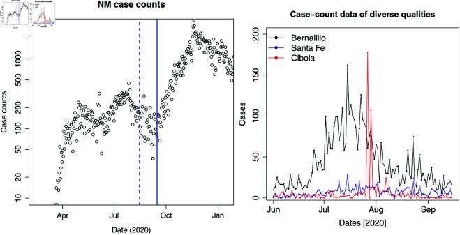
In this paper, we present a method for estimating the infection-rate of a disease as a spatial-temporal field. Our data comprises time-series case-counts of symptomatic patients in various areal units of a region. We extend an epidemiological model, originally designed for a single areal unit, to accommodate multiple units. The field estimation is framed within a Bayesian context, utilizing a parameterized Gaussian random field as a spatial prior. We apply an adaptive Markov chain Monte Carlo method to sample the posterior distribution of the model parameters condition on COVID-19 case-count data from three adjacent counties in New Mexico, USA. Our results suggest that the correlation between epidemiological dynamics in neighboring regions helps regularize estimations in areas with high variance (i.e., poor quality) data. Using the calibrated epidemic model, we forecast the infection-rate over each areal unit and develop a simple anomaly detector to signal new epidemic waves. Our findings show that anomaly detector based on estimated infection-rates outperforms a conventional algorithm that relies solely on case-counts.


Conflict of interest statement

The authors have declared that no competing interests exist.

Figures

Fig 1
Fig 1. Left: The waves of COVID-19 infection in New Mexico in 2020.
The data from the “Summer wave” (June 1, 2020 to September 15, 2020) will be used to estimate the infection-rate field. The Fall 2020 wave started around September 15, and is marked with a solid vertical line. The dashed line is August 15. Right: Case-count data during the “Summer wave” for 3 counties. Note the erroneous data spikes in the middle of the summer for Cibola. Data quality for the various areal units can vary significantly.
Fig 2
Fig 2. Top left: Evolution of coefficients wk,t over time as the risk-factor model is fitted to cumulative case-counts yt,r normalized by county populations.
Results are plotted for the intercept and four principal components (PC). Only the intercept survives and is far larger that the weights associated with the principal components. Top right: Plot of the prediction error from a 7-fold cross-validation performed with the risk-factor model and LASSO, on case-count data accumulated over the entire two-and-a-half-year duration (and normalized by county populations). The figures on the upper horizontal axis denotes the number of principal components retained in the fitted model. λmin and λ1se are clearly marked. Bottom left: Distribution of coefficients, corresponding to penalties λmin and λ1se; the intercept dominates. Bottom right: The residuals from the risk-factors model i.e., the component not explained by the risk-factors model. The spatial correlations are clear.
Fig 3
Fig 3. The geographical extent of three adjacent New Mexico counties considered in this paper: Bernalillo (in green), Santa Fe (in red) and Valencia (in blue).
Fig 4
Fig 4. 1-D marginal posterior distributions to Bernalillo (left column), Santa Fe (middle column), and Valencia (right column).
Top row: PDFs for t0,r. t0,r values are negative as it is measured from June 10th, 2020, and the PDFs imply that infections for the Summer wave started in late May. Second row: PDFs for Nr. Third row: PDFs for k. Bottom row: PDFs for θr.
Fig 5
Fig 5. Marginal posterior distributions for GMRF parameters (τϕ2,λϕ) (top row) and noise parameters (σa,σm) (bottom row), estimated via 2r and 3r joint estimations with data for Santa Fe.
Fig 6
Fig 6. Comparison of posterior predictive distribution results obtained via joint inference (using the GMRF model) for Bernalillo (left), Santa Fe (middle), and Valencia (right) shown on top row with equivalent results from independent inferences for each county separately, on the bottom row; data up to September 15th, 2020 is used and case-count data (shown with black circles) was smoothed with a 7-day running average.
The red line is the median prediction, the shaded teal region is the inter-quartile range and the dashed lines are 5th and 95th percentiles and the white circles are actual counts in the forecast regime.
Fig 7
Fig 7. Comparison of reconstructed infection-rate profiles that underlie the predictions in Fig 6.
The top row contains results obtained via joint inference (using the GMRF model) for Bernalillo (left), Santa Fe (middle), and Valencia (right). Results from independent inferences for each county separately, are shown in the bottom row. The calibration data spans up to September 15th, 2020 and the case-count data was smoothed with a 7-day running average. The red line is the median prediction, the shaded teal region is the inter-quartile range and the dashed lines are 5th and 95th percentiles. difference is not the consequence of over-smoothing in time by our “mechanistic” treatment of time-evolution of the outbreak vis-à-vis a pCAR-ST model, which would likely employ an auto-regressive or moving-average approach. In Fig 7, we plot the corresponding infection-rates for all three counties. Differences in the estimated infection-rates, 3r joint estimation (top row) versus independent (bottom row), are difficult to discern. This is because the infection-rate is only affected by (t0,r,kr,Nr,θr) and, as is clear from Fig 4, there is not much difference in their posterior PDFs. Instead, it is the noise and spatial parameters whose estimates differ as we add more regions to the joint estimation (see Fig 5).
Fig 8
Fig 8. Infection-rate detector results (top row) compared with the GLR-Poisson detector (bottom row), using data from 2020-06-01 to 2020-09-15.
The symbols are the observed case-counts for Bernalillo (left), Santa Fe (middle), and Valencia (right). The Fall 2020 wave is believed to have started around September 15. The red line beyond September 15 is the outlier boundary; a day with a case-count above the dashed line is an “outlier” and is circled. A data point with a square box around it denotes the the last of a sequence of three consecutive alarmed days. In all cases we see that the GLR-Poisson detector misses the Fall 2020 wave.
Fig 9
Fig 9. Variation explained by the principal components obtained via sparse PCA of the 79 risk factors used to model population-normalized case-counts in the counties of New Mexico.
We see that 12 principal components can cover 95% of the variations observed in the risk-factors.
Fig 10
Fig 10. Infection-rate detector results (top row) compared with the GLR-Poisson detector (bottom row), using data from 2020-06-01 to 2020-08-15.
August 15 is a month before the arrival of the Fall 2020 wave. Lines and symbols’ settings are the same as in Fig 8. We see that for Bernalillo and Santa Fe, both methods suffer from false positives, detecting alarms before the arrival of the Fall 2020 wave.
Fig 11
Fig 11. One and two-dimensional marginal posterior distributions for the Bernalillo county model parameters; left: 3 region joint inversion, right: Bernalillo county only.
Fig 12
Fig 12. One and two-dimensional marginal posterior distributions for the Santa Fe county model parameters; left: 3 region joint inversion, right: Santa Fe county only.
Fig 13
Fig 13. One and two-dimensional marginal posterior distributions for the Valencia county model parameters; left: 3 region joint inversion, right: Valencia county only.

Similar articles

  • The effect of sample site and collection procedure on identification of SARS-CoV-2 infection.
    Davenport C, Arevalo-Rodriguez I, Mateos-Haro M, Berhane S, Dinnes J, Spijker R, Buitrago-Garcia D, Ciapponi A, Takwoingi Y, Deeks JJ, Emperador D, Leeflang MMG, Van den Bruel A; Cochrane COVID-19 Diagnostic Test Accuracy Group. Davenport C, et al. Cochrane Database Syst Rev. 2024 Dec 16;12(12):CD014780. doi: 10.1002/14651858.CD014780. Cochrane Database Syst Rev. 2024. PMID: 39679851 Free PMC article.
  • ScITree: Scalable Bayesian inference of transmission tree from epidemiological and genomic data.
    Waddel H, Koelle K, Lau MSY. Waddel H, et al. PLoS Comput Biol. 2025 Jun 10;21(6):e1012657. doi: 10.1371/journal.pcbi.1012657. eCollection 2025 Jun. PLoS Comput Biol. 2025. PMID: 40493703 Free PMC article.
  • Signs and symptoms to determine if a patient presenting in primary care or hospital outpatient settings has COVID-19.
    Struyf T, Deeks JJ, Dinnes J, Takwoingi Y, Davenport C, Leeflang MM, Spijker R, Hooft L, Emperador D, Domen J, Tans A, Janssens S, Wickramasinghe D, Lannoy V, Horn SRA, Van den Bruel A; Cochrane COVID-19 Diagnostic Test Accuracy Group. Struyf T, et al. Cochrane Database Syst Rev. 2022 May 20;5(5):CD013665. doi: 10.1002/14651858.CD013665.pub3. Cochrane Database Syst Rev. 2022. PMID: 35593186 Free PMC article.
  • Rapid, point-of-care antigen tests for diagnosis of SARS-CoV-2 infection.
    Dinnes J, Sharma P, Berhane S, van Wyk SS, Nyaaba N, Domen J, Taylor M, Cunningham J, Davenport C, Dittrich S, Emperador D, Hooft L, Leeflang MM, McInnes MD, Spijker R, Verbakel JY, Takwoingi Y, Taylor-Phillips S, Van den Bruel A, Deeks JJ; Cochrane COVID-19 Diagnostic Test Accuracy Group. Dinnes J, et al. Cochrane Database Syst Rev. 2022 Jul 22;7(7):CD013705. doi: 10.1002/14651858.CD013705.pub3. Cochrane Database Syst Rev. 2022. PMID: 35866452 Free PMC article.
  • Antibody tests for identification of current and past infection with SARS-CoV-2.
    Fox T, Geppert J, Dinnes J, Scandrett K, Bigio J, Sulis G, Hettiarachchi D, Mathangasinghe Y, Weeratunga P, Wickramasinghe D, Bergman H, Buckley BS, Probyn K, Sguassero Y, Davenport C, Cunningham J, Dittrich S, Emperador D, Hooft L, Leeflang MM, McInnes MD, Spijker R, Struyf T, Van den Bruel A, Verbakel JY, Takwoingi Y, Taylor-Phillips S, Deeks JJ; Cochrane COVID-19 Diagnostic Test Accuracy Group. Fox T, et al. Cochrane Database Syst Rev. 2022 Nov 17;11(11):CD013652. doi: 10.1002/14651858.CD013652.pub2. Cochrane Database Syst Rev. 2022. PMID: 36394900 Free PMC article.

References

    1. Daza-Torres ML, Capistrán MA, Capella A, Christen JA. Bayesian sequential data assimilation for COVID-19 forecasting. Epidemics. 2022;39:100564. doi: 10.1016/j.epidem.2022.100564 - DOI - PMC - PubMed
    1. Wang Z, Zhang X, Teichert GH, Carrasco-Teja M, Garikipati K. System inference for the spatio-temporal evolution of infectious diseases: Michigan in the time of COVID-19. Comput Mech. 2020;66(5):1153–76. doi: 10.1007/s00466-020-01894-2 - DOI - PMC - PubMed
    1. Chen P, Wu K, Ghattas O. Bayesian inference of heterogeneous epidemic models: application to COVID-19 spread accounting for long-term care facilities. Comput Methods Appl Mech Eng. 2021;385:114020. doi: 10.1016/j.cma.2021.114020 - DOI - PMC - PubMed
    1. Blonigan P, Ray J, Safta C. Forecasting multi-wave epidemics through Bayesian inference. Arch Comput Methods Eng. 2021;28(6):4169–83. doi: 10.1007/s11831-021-09603-9 - DOI - PMC - PubMed
    1. Lin YT, Neumann J, Miller EF, Posner RG, Mallela A, Safta C, et al. Daily forecasting of regional epidemics of coronavirus disease with bayesian uncertainty quantification, United States. Emerg Infect Dis. 2021;27(3):767–78. doi: 10.3201/eid2703.203364 - DOI - PMC - PubMed