Rapid, interpretable data-driven models of neural dynamics using recurrent mechanistic models

Abstract

Obtaining predictive models of a neural system is notoriously challenging. Detailed models suffer from excess model complexity and are difficult to fit efficiently. Simplified models must negotiate a tradeoff between tractability, predictive power, and ease of interpretation. We present a modeling paradigm for estimating predictive, mechanistic models of neurons and small circuits that navigates these issues using methods from systems theory. The key insight is that membrane currents can be modeled using two scalable system components optimized for learning: linear state space models, and nonlinear artificial neural networks. Combining these components, we construct two types of membrane currents: lumped currents, which are flexible, and data-driven conductance-based currents, which are interpretable. The resulting class of models-which we call recurrent mechanistic models (RMMs)-can be trained in a matter of seconds to minutes on intracellular recordings during an electrophysiology experiment, representing a step change in performance over previous approaches. As a proof-of-principle, we use RMMs to learn the dynamics of two groups of neurons, and their synaptic connections, in the Stomatogastric Ganglion, a well-known central pattern generator. Due to their reliability, efficiency, and interpretability, RMMs enable qualitatively new kinds of experiments using predictive models in closed-loop neurophysiology and online estimation of neural properties in living preparations.

Keywords: biophysical models; central pattern generators; electrophysiology; machine learning; neural dynamics.

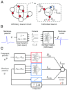
Fig. 1.

(A) Recurrent mechanistic models (RMMs) are designed to rapidly infer the excitable dynamics of neural circuits from measured physiological variables. This paper focuses on intracellular membrane voltages; accordingly, each neuron in the circuit integrates synaptic (red) and intrinsic (blue) ionic currents. (B) Synaptic and intrinsic currents are obtained by filtering a neuron’s membrane voltage through a state space system, whose outputs (features) are then recombined by an ANN. State-space systems can be systematically designed to have orthogonal convolution kernels, resulting in dynamically rich features for the ANNs to recombine (Methods). Modeling flexibility can be traded off for interpretability by imposing architectural constraints on the ANN. (C) An excitable neuron model is obtained by integrating applied, intrinsic and synaptic membrane currents. The blocks depicted in color are those containing the main trainable parameters of the model, which also include the membrane capacitance, c. While state space models can in principle be learned, biophysical intuition can be used to construct them and keep them fixed, leading to faster training times (Methods). Dots indicate time derivatives; in practice, the model is implemented in discrete-time.

Fig. 2.

RMMs recover the classical Hodgkin–Huxley conductances (21) from input–output data. (A) A state space system with eight internal states is designed so that the states evolve in fast and slow timescales roughly corresponding to those of the spiking dynamics of the original HH model. The ANN-based readout is constrained to promote interpretability (cf. Fig. 1): Sodium and potassium conductances are obtained as outputs of MLPs, and the corresponding ionic currents are obtained by multiplying those data-driven conductances by a difference in potential $(v-E_{\text{ion}})$, with $E_{\text{ion}}$ a prior reversal potential. To ensure the model learns the correct currents, fixed layers selecting fast and slow states are used. (B) Target voltage trace (Top) resulting from simulating the original HH model given a noisy applied current, and corresponding RMM prediction (Bottom) on held-out test data. (C) (Top) zoom of the dashed region in (B) shows accuracy of spike prediction. (Middle, Bottom) The RMM accurately recovers conductance trajectories during spiking. For modeling and training details, see Hodgkin–Huxley RMM.

Fig. 3.

Estimating an RMM of a neuron with complex spatiotemporal dynamics. (A) Experimental setup used to generate data for fitting an RMM: The STG circuit is bathed in PTX, which blocks Glutamate synapses but not Acetylcholine synapses; intracellular recordings are taken of one of the PD neurons and the LP neuron; the resulting system is a feedforward interconnection with the measured presynaptic PD neuron voltage driving the LP neuron. (B) Example voltage traces showing held-out data (three Top panels) and the predicted voltage and synaptic currents from an RMM trained with teacher forcing (TF). (C) Evolution of loss functions during rapid training with TF and multiple-shooting (MS): Three different trial datasets are shown; the blue Trial 1 yields the model used as example in (B); predictions of the models trained on Trials 2 and 3 are shown in SI Appendix, Fig. S2. Each training dataset consists of around 96 s of data recorded with a sampling period of 0.1 ms. Top: TF loss function during training; Middle: validation loss function using models trained with TF (evaluated with held-out data); Bottom: MS improves the performance of the best model obtained with TF. Training RMMs with TF avoids backpropagation through time, which is employed in MS in a limited fashion (Methods). (D) Example traces demonstrating the improvement obtained with multiple shooting.

Fig. 4.

Training an RMM with lumped and mechanistic currents to learn endogenous bursting rhythms. (A) diagram of the AB-PD pacemaker dynamics, simplified here as a single PD cell (29). Fitting traditional mechanistic models to the system is challenging: A single-compartment conductance-based model cannot quantitatively predict the membrane voltage at the soma (where recordings are made), since fast currents are located in a distant part of the axon. (B) To quickly obtain a predictive single-compartment model, we employ an RMM with a mix of lumped and mechanistic currents. The lumped current, which does not distinguish between ion channels, is used to predict the fast axonal current. To model the ionic currents of the soma, we employ three data-driven mechanistic currents to capture the aggregate dynamics of potassium, calcium, and hyperpolarization-induced currents. (C) Validation of an RMM on held-out membrane voltage data (black traces). The model, which was trained on current-clamp data (Methods) predicts the membrane voltage well. In addition, the model allows interpreting its internal variables as individual currents and conductances. SI Appendix, Fig. S5 shows similar results for four different PD neuron preparations, and SI Appendix, Fig. S6 shows associated learning curves. (D) Steady-state IV curves of each of the RMM intrinsic currents, averaged over 18 satisfactory models trained with different dataset batches and different random parameter initialization seeds. The IV curves show consistency in RMM biophysical features after training. (E) Removing the fast lumped current from the RMM uncovers the slow wave dynamics underlying burst excitability. Models were trained with teacher forcing (Methods) over 200 epochs, corresponding to about two minutes of training over 168-s long dataset batches.

References

1. Paninski L., Pillow J., Simoncelli E., Comparing integrate-and-fire models estimated using intracellular and extracellular data. Neurocomputing 65, 379–385 (2005).
1. Abarbanel H., Creveling D., Farsian R., Kostuk M., Dynamical state and parameter estimation. SIAM J. Appl. Dyn. Syst. 8, 1341–1381 (2009).
1. Meliza C. D., et al. , Estimating parameters and predicting membrane voltages with conductance-based neuron models. Biol. Cybern. 108, 495–516 (2014). - PubMed
1. J. M. Lueckmann et al. , “Flexible statistical inference for mechanistic models of neural dynamics” in 31st Conference on Neural Information Processing Systems (NIPS 2017), I. Guyon et al. , Eds. (Long Beach, CA, USA, 2017), pp. 1289–1299.
1. Abu-Hassan K., et al. , Optimal solid state neurons. Nat. Commun. 10, 5309 (2019). - PMC - PubMed
LinkOut - more resources