. 2025 Aug 4:6:0336.
doi: 10.34133/cbsystems.0336. eCollection 2025.

Dynamic Network Plasticity and Sample Efficiency in Biological Neural Cultures: A Comparative Study with Deep Reinforcement Learning

Affiliations

Dynamic Network Plasticity and Sample Efficiency in Biological Neural Cultures: A Comparative Study with Deep Reinforcement Learning

Moein Khajehnejad et al. Cyborg Bionic Syst. .

Abstract

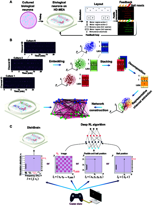
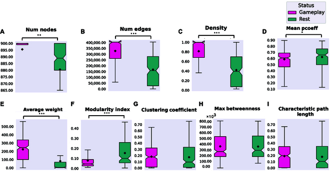
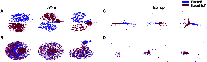
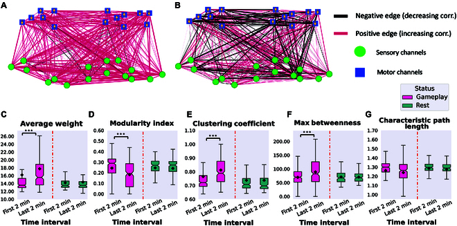
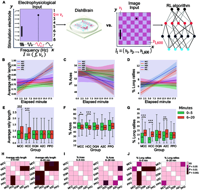
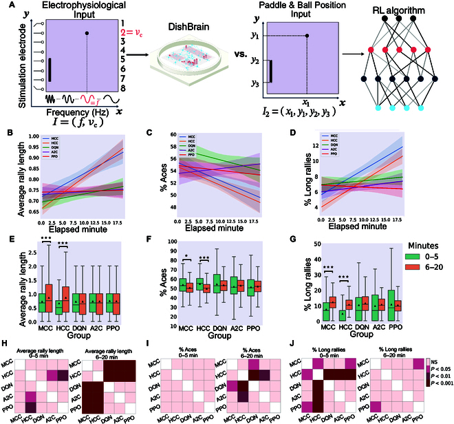
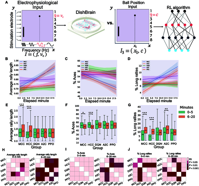
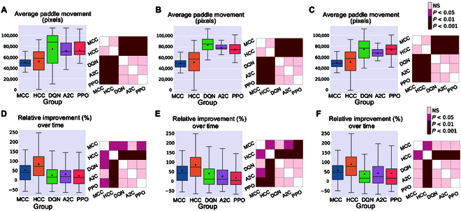
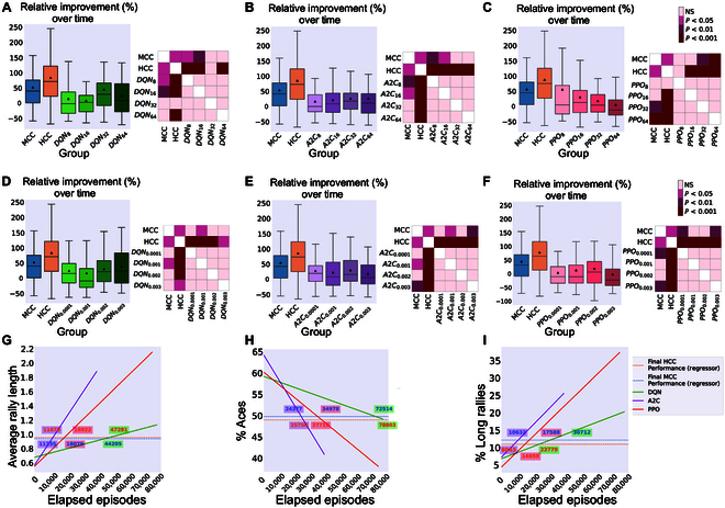
In this study, we investigate the complex network dynamics of in vitro neural systems using DishBrain, which integrates live neural cultures with high-density multi-electrode arrays in real-time, closed-loop game environments. By embedding spiking activity into lower-dimensional spaces, we distinguish between spontaneous activity (Rest) and Gameplay conditions, revealing underlying patterns crucial for real-time monitoring and manipulation. Our analysis highlights dynamic changes in connectivity during Gameplay, underscoring the highly sample efficient plasticity of these networks in response to stimuli. To explore whether this was meaningful in a broader context, we compared the learning efficiency of these biological systems with state-of-the-art deep reinforcement learning (RL) algorithms (Deep Q Network, Advantage Actor-Critic, and Proximal Policy Optimization) in a simplified Pong simulation. Through this, we introduce a meaningful comparison between biological neural systems and deep RL. We find that when samples are limited to a real-world time course, even these very simple biological cultures outperformed deep RL algorithms across various game performance characteristics, implying a higher sample efficiency.


Conflict of interest statement

Competing interests: B.J.K., A.L., F.H., and M.K. were contracted or employed by Cortical Labs during the course of this research. B.J.K. has shares in Cortical Labs and an interest in patents related to this work. All other authors declare that they have no competing interests.

Figures

Fig. 1.
Fig. 1.
(A) Schematic illustration of the DishBrain feedback loop, the simulated game environment, and electrode configurations. (B) A schematic illustration of the overall network construction framework. The spiking time series data are first transformed into a 3D space using t-SNE embedding. These lower-dimensional representations are then combined into a tensor, which is decomposed using Tucker decomposition. The K-medoids algorithm is then applied to identify consistent representative channels across all cultures. These channels become network nodes, and pairwise Pearson correlation values serve as edge weights. The network layout reflects the physical placement of channels on the MEA, with node colors distinguishing sensory (green) from motor (blue) regions. (C) Schematic comparing the information input routes in the DishBrain system (left) and the 3 implementations of the deep RL algorithms (right). In each design, the input information to the computing module (deep RL algorithms or DishBrain) is denoted by a vector I. Note that in the DishBrain system, while this figure depicts stylized waveforms for illustrative purposes, the actual stimulation consisted of discrete electrical pulses.
Fig. 2.
Fig. 2.
Significant network plasticity occurs in biological cultures when embodied in the game environment. (A to I) Network summary statistics of 1,024 recorded channels using the full duration of all Gameplay and Rest sessions. Using one-way t tests, we found significant differences in the number of nodes (P = 3.072e−3), number of edges (P = 8.396e−26), density (P = 1.009e−25), mean participation coefficient (pcoeff) (P = 3.400e−2), average weight (P = 8.910e−20), and modularity index (P = 4.129e−13) between Gameplay and Rest. No significant differences were found for clustering coefficient (P = 0.568), max betweenness (P = 0.890), or characteristic path length (P = 0.533).
Fig. 3.
Fig. 3.
Low-dimensional representation of 3 samples of (A) Gameplay sessions and their following (B) Rest sessions using t-SNE as well as (C) Gameplay sessions and their following (D) Rest sessions using Isomap. The purple and maroon dots are the channel representations in the embedding space in the first and second halves of the recordings, respectively. Both dimensionality reduction algorithms were able to distinguish between the 2 halves of recording during Gameplay but not during Rest sessions.
Fig. 4.
Fig. 4.
The average connectivity networks using 30 representative channels over all (A) Gameplay and (B) Rest sessions with edge weights representing changes in functional connectivity between channel pairs when comparing the last 2 min to the first 2 min of recordings. Edge colors signify the direction of these connectivity changes, with red indicating increases and black indicating decreases. Motor and sensory region channels are represented by blue squares and green circles, respectively. Arrows on motor region nodes show the paddle’s movement direction as per their position in the predefined layout in Fig. 1. (C to G) Network summary statistics between the first and last 2 min of Gameplay and Rest recordings using the 30 representative channels in the lower-dimensional space. All of these metrics except the characteristic path length showed statistically significant differences using one-way ANOVA during Gameplay (P = 2.265e−3, P = 8.478e−8, P = 1.891e−6, P = 1.005e−4, and P = 0.071, respectively), but not in the Rest condition of the cultures (P = 0.864, P = 0.670, P = 0.738, P = 0.281, and P = 0.899, respectively). ***P < 0.001.
Fig. 5.
Fig. 5.
Image Input to the deep RL algorithms. (A) Schematic highlighting figure comparisons are between biological DishBrain system and a pixel-based information input to the RL algorithms. Average number of (B) hits-per-rally, (C) % of aces, and (D) % of long rallies over 20 min real-time equivalent of training DQN, A2C, PPO, MCC, and HCC cultures. A regressor line on the mean values with a 95% confidence interval highlights the learning trends. Comparing the performance among all groups, the highest level of average hits-per-rally is achieved by the neural MCC and HCC cultures while PPO is outperformed by all the opponents. The average % of aces is lowest for the neural cultures compared to all deep RL baseline methods. The average % of long rallies reaches its highest levels for MCC and HCC. (E) Average performance of groups over time. Only biological cultures have significant within-group improvement and increase in their performance at the second time interval (one-way ANOVA test, P = 5.854e−6 and P = 7.936e−17 for MCC and HCC, respectively; P = 0.231, P = 0.318, and P = 0.400 for DQN, A2C, and PPO respectively). (F) Average % of aces within groups and over time. Only MCC and HCC (one-way ANOVA test, P = 0.014 and P = 2.907e−8, respectively) differed significantly over time. No significant change was detected within the DQN, A2C, or PPO groups (one-way ANOVA test, P = 0.080, P = 0.195, and P = 0.308, respectively). (G) Average % of long-rallies (≥3) performed in a session. All groups showed an increase in the average number of long rallies where this within-group increase was significant only for MCC, HCC, and A2C (one-way ANOVA test, P = 1.172e−7 and P = 1.525e−24 for MCC and HCC, respectively and P = 0.605, P = 0.002, and P = 0.684 for DQN, A2C, and PPO, respectively). *P < 0.05, **P < 0.01, and ***P < 0.001. (H) Pairwise Tukey’s post-hoc test shows that HCC and MCC groups significantly outperform PPO, A2C, and DQN in the last 15-min interval. (I) Using pairwise Tukey’s post-hoc test, the HCC group significantly outperforms the PPO in the last 15-min interval with a lower average of % Aces. A2C also outperforms PPO in this time interval. (J) Pairwise comparison using Tukey’s test only shows a significant difference in the percentage of long rallies between HCC and the rest of the groups in the first 5 min. However, this is later altered in the direction of all groups having an increased % of long rallies with MCC outperforming PPO in the last 15 min of the game. Box plots show interquartile range, with bars demonstrating 1.5× interquartile range; the line marks the median and the black triangle marks the mean. Error bands = 1 SE.
Fig. 6.
Fig. 6.
Paddle & Ball Position Input to the deep RL algorithms. (A) Schematic highlighting figure comparisons are between biological DishBrain system and Paddle & Ball Position Input to RL algorithms. Average number of (B) hits-per-rally, (C) % of aces, and (D) % of long rallies over 20 min real-time equivalent of training DQN, A2C, PPO, MCC, and HCC cultures. A regressor line on the mean values with a 95% confidence interval highlights the learning trends. The highest level of average hits-per-rally is achieved by the MCC and HCC cultures. The average % of aces is lowest for the neural cultures compared to all deep RL baseline methods. The average % of long rallies reaches its highest levels for MCC and HCC. (E) Average rally length over time only showed a significant increase in the biological cultures between the 2 time intervals (one-way ANOVA test, P = 0.913, P = 0.958, and P = 0.610 for DQN, A2C, and PPO, respectively). (F) Average % of aces within groups and over time only showed a significant difference in the MCC and HCC groups. No significant change was detected within the DQN, A2C, or PPO groups (one-way ANOVA test, P = 0.463, P = 0.338, and P = 0.544, respectively). (G) Average % of long-rallies (≥3) performed in a session increased in the second time interval in all groups. This within-group difference was only significant for the MCC and HCC groups (one-way ANOVA test, P = 1.172e−7, P = 1.525e−24, P = 0.233, P = 0.320, and P = 0.650 for MCC, HCC, DQN, A2C, and PPO, respectively). *P < 0.05 and ***P < 0.001. (H) Pairwise Tukey’s post-hoc test shows that the HCC group is significantly outperformed by A2C and PPO in the first 5 min in terms of the hit counts. Biological cultures, however, do significantly better compared to all deep RL opponents in the 15-min interval. (I) Using pairwise Tukey’s post-hoc test, the HCC group significantly outperforms the DQN and A2C groups in the last 15-min interval with a lower average of % Aces. DQN is also outperformed by the MCC group in this time interval. (J) Pairwise comparison using Tukey’s test shows a significant difference in the percentage of long rallies between HCC and the rest of the groups in the first 5 min all outperforming the HCC. However, this is later altered in the last 15 min with only MCC outperforming PPO significantly having an increased % of long rallies. Box plots show interquartile range, with bars demonstrating 1.5× interquartile range; the line marks the median and the black triangle marks the mean. Error bands = 1 SE.
Fig. 7.
Fig. 7.
Ball Position Input to the deep RL algorithms. (A) Schematic highlighting figure comparisons are between biological DishBrain system and Ball Position Input to RL algorithms. Average number of (B) hits-per-rally, (C) % of aces, and (D) % of long rallies over 20 min real-time equivalent of training DQN, A2C, PPO, MCC, and HCC cultures. A regressor line on the mean values with a 95% confidence interval highlights the learning trends. The highest level of average hits-per-rally is achieved by the neural MCC and HCC cultures. The average % of aces is lowest for the neural cultures compared to all deep RL baseline methods. The average % of long rallies reaches its highest levels for MCC and HCC. Comparing to the same findings for the HCC and MCC groups, (E) average rally length over time only showed a significant increase in the biological cultures between the 2 time intervals (one-way ANOVA test, P = 0.995, P = 0.812, and P = 0.547 for DQN, A2C, and PPO, respectively). (F) Average % of aces within groups and over time only showed a significant difference in the MCC and HCC groups. No significant change was detected within the DQN, A2C, or PPO groups (one-way ANOVA test, P = 0.241, P = 0.581, and P = 0.216, respectively). (G) Average % of long rallies (≥3) performed in a session increased in the second time interval in all groups except DQN. This within-group difference was only significant for MCC, HCC, and A2C groups with P = 0.002 for the A2C group. *P < 0.05, **P < 0.01, and ***P < 0.001. (H) Pairwise Tukey’s post-hoc test shows that biological cultures significantly outperform all deep RL groups in the last 15 min in terms of the hit counts or rally length. (I) Using pairwise Tukey’s post-hoc test, the HCC group significantly outperforms all the deep RL groups in the last 15-min interval while MCC also outperforms DQN with a lower average of % Aces. (J) Pairwise comparison using Tukey’s test shows a significant out-performance of all groups over HCC in the percentage of long rallies in the first 5 min. In the second time interval, MCC shows a significantly higher % of long rallies compared to DQN with HCC now being outperformed only by A2C. Box plots show interquartile range, with bars demonstrating 1.5× interquartile range; the line marks the median and the black triangle marks the mean. Error bands = 1 SE.
Fig. 8.
Fig. 8.
Paddle movement and relative improvement. The average paddle movement in pixels in all the different groups for the (A) Image Input, (B) Paddle & Ball Position Input, and (C) Ball Position Input to the deep RL algorithms. Tukey’s post-hoc test was conducted showing that DQN, PPO, and A2C had a significantly higher average paddle movement compared to HCC and MCC in all scenarios. Relative improvement (%) in the average hit counts between the first 5 min and the last 15 min of all sessions in each separate group for the (D) Image Input, (E) Paddle & Ball Position Input, and (F) Ball Position Input to the deep RL algorithms. The biological groups show higher improvements with HCC outperforming all. (D) Using Games Howell post-hoc test, the inter-group differences were significant with HCC outperforming all other groups, as well as MCC significantly outperforming PPO. (E) HCC showed a significantly higher relative improvement compared to all the other groups while MCC also outperformed A2C and PPO in terms of relative improvement over time. (F) Finally, HCC could still perform significantly better than all the deep RL groups with the Ball Position Input design to the deep RL algorithms with MCC outperforming PPO and DQN in this design.
Fig. 9.
Fig. 9.
Batch size and learning rate effects for the RL algorithms with Image Input. Relative improvement (%) in the average hit counts between the first 5 min and the last 15 min of all sessions as well as the post-hoc tests in each separate group for batch sizes of 8, 16, 32, and 64 in the (A) DQN, (B) A2C, and (C) PPO groups compared to biological cultures. Games Howell post-hoc tests show the inter-group differences that were not significant between any pair of different batch sizes for any of the DQN, A2C, or PPO groups. Relative improvement (%) in the average hit counts between the first 5 min and the last 15 min of all sessions for learning rate (critic learning rate for PPO and A2C algorithms) values of 0.0001, 0.001, 0.002, and 0.003 in the (D) DQN, (E) A2C, and (F) PPO groups compared to biological cultures. Games Howell post-hoc tests show the inter-group differences that were not significant between any pair of different batch sizes for any of the DQN, A2C, or PPO groups while the HCC group significantly outperforms all RL algorithms in this measure. (G to I) Extended training episodes for the deep RL algorithms. Illustrating the performance of a single DQN, A2C, and PPO with the Image Input over an extended number of training episodes, measured in terms of (G) average rally length, (H) % of aces, and (I) % of long rallies. The final performance levels of the HCC and MCC groups are shown with dashed horizontal lines, and the episode numbers at which these RL algorithms surpass these levels are annotated on the plots.

Similar articles

Cited by

References

    1. Ramchandran K, Zeien E, Andreasen NC. Distributed neural efficiency: Intelligence and age modulate adaptive allocation of resources in the brain. Trends Neurosci Educ. 2019;15:48–61. - PubMed
    1. Kudithipudi D, Aguilar-Simon M, Babb J, Bazhenov M, Blackiston D, Bongard J, Brna AP, Raja SC, Cheney N, Clune J, et al. Biological underpinnings for lifelong learning machines. Nat Mach Intell. 2022;4(3):196–210.
    1. Lake BM, Ullman TD, Tenenbaum JB, Gershman SJ. Building machines that learn and think like people. Behav Brain Sci. 2017;40: Article e253. - PubMed
    1. Hassabis D, Kumaran D, Summerfield C, Botvinick M. Neuroscience-inspired artificial intelligence. Neuron. 2017;95(2):245–258. - PubMed
    1. Sutton RS, Barto AG. Reinforcement learning: An introduction. MIT Press; 2018.

LinkOut - more resources