Distilling knowledge from graph neural networks trained on cell graphs to non-neural student models

Abstract

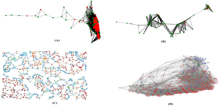
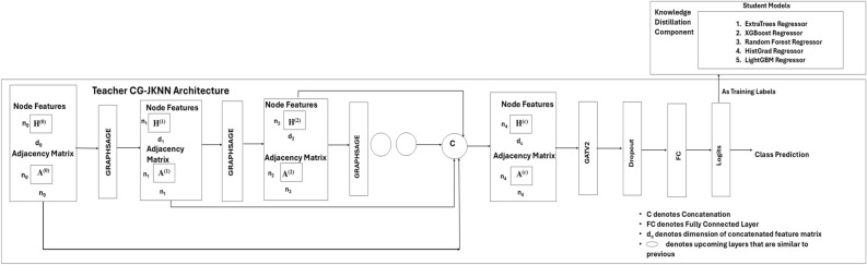
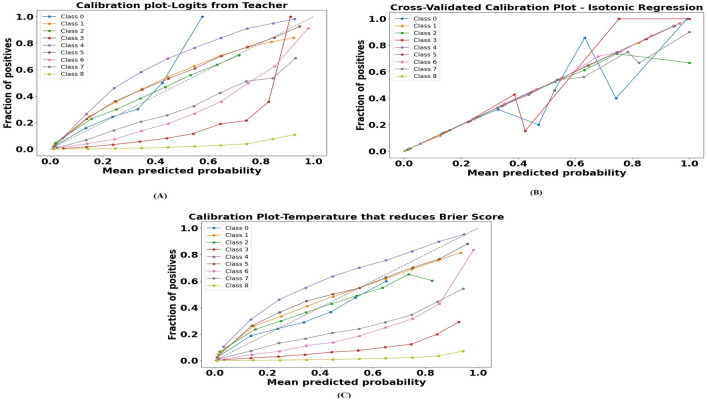
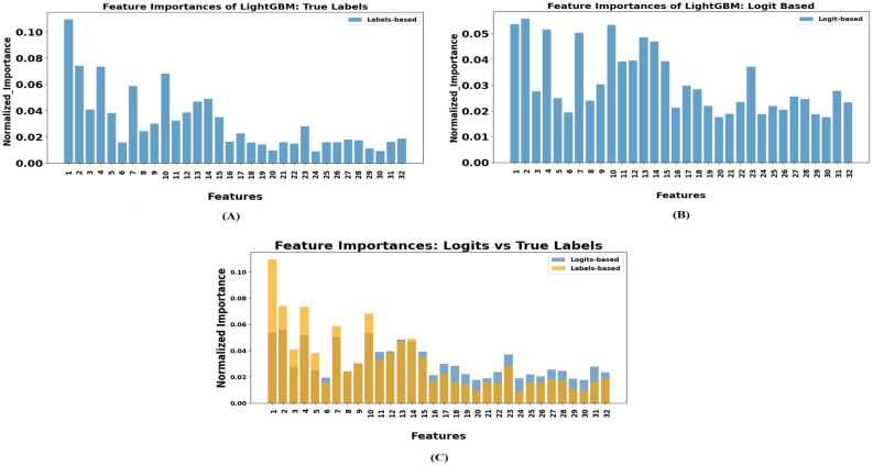
The development and refinement of artificial intelligence (AI) and machine learning algorithms have been an area of intense research in radiology and pathology, particularly for automated or computer-aided diagnosis. Whole Slide Imaging (WSI) has emerged as a promising tool for developing and utilizing such algorithms in diagnostic and experimental pathology. However, patch-wise analysis of WSIs often falls short of capturing the intricate cell-level interactions within local microenvironment. A robust alternative to address this limitation involves leveraging cell graph representations, thereby enabling a more detailed analysis of local cell interactions. These cell graphs encapsulate the local spatial arrangement of cells in histopathology images, a factor proven to have significant prognostic value. Graph Neural Networks (GNNs) can effectively utilize these spatial feature representations and other features, demonstrating promising performance across classification tasks of varying complexities. It is also feasible to distill the knowledge acquired by deep neural networks to smaller student models through knowledge distillation (KD), achieving goals such as model compression and performance enhancement. Traditional approaches for constructing cell graphs generally rely on edge thresholds defined by sparsity/density or the assumption that nearby cells interact. However, such methods may fail to capture biologically meaningful interactions. Additionally, existing works in knowledge distillation primarily focus on distilling knowledge between neural networks. We designed cell graphs with biologically informed edge thresholds or criteria to address these limitations, moving beyond density/sparsity-based definitions. Furthermore, we demonstrated that student models do not need to be neural networks. Even non-neural models can learn from a neural network teacher. We evaluated our approach across varying dataset complexities, including the presence or absence of distribution shifts, varying degrees of imbalance, and different levels of graph complexity for training GNNs. We also investigated whether softened probabilities obtained from calibrated logits offered better guidance than raw logits. Our experiments revealed that the teacher's guidance was effective when distribution shifts existed in the data. The teacher model demonstrated decent performance due to its higher complexity and ability to use cell graph structures and features. Its logits provided rich information and regularization to students, mitigating the risk of overfitting the training distribution. We also examined the differences in feature importance between student models trained with the teacher's logits and their counterparts trained on hard labels. In particular, the student model demonstrated a stronger emphasis on morphological features in the Tuberculosis (TB) dataset than the models trained with hard labels. This emphasis aligns closely with the features that pathologists typically prioritize for diagnostic purposes. Future work could explore designing alternative teacher models, evaluating the proposed approach on larger datasets, and investigating causal knowledge distillation as a potential extension.

Keywords: Cell graphs; Graph neural networks; Knowledge distillation; Non-neural models; Tuberculosis; Whole slide imaging.

Figure 1

Cell graphs of the TB and BRCA-M2C datasets were generated using the NetworkX library (version 3.4.2, https://networkx.org/). (A) Cell Graph generated for a TB image. Acid-fast bacilli (AFB) cells are shown in red, and the nucleus of activated macrophages is depicted in blue. Black edges represent interactions. (B) Cell Graph generated for a normal lung tissue, i.e., not infected. (C) Cell Graph acquired from the Vanea et al., licensed under Creative Commons Attribution 4.0 International License (https://creativecommons.org/licenses/by/4.0/). (D) Cell Graph generated from the BRCA-M2C dataset, where red nodes represent lymphocytes, blue nodes represent tumor cells, green nodes represent stromal cells, and gray edges denote their interactions, created using different k-values for specific cell interactions.

Figure 2

Architecture of the teacher model used for knowledge distillation. To obtain the temperature-scaled logits, as discussed in the ablation study, a temperature-scaling block needs to be incorporated between the logits generated by the teacher model and the input to the student models.

Algorithm 1

Optimal Weight Finding for Ensemble of Teacher GNN and Best Student model

Figure 3

Architecture of our shallow ANN student model. The ellipses denote that additional neurons are present in the layer but are not explicitly illustrated for clarity.

Figure 4

Calibration plot of raw logits converted to probabilities for positive class-TB dataset.

Figure 5

Performance of best performing student models and their counterparts on the test set-TB. We see student models outperforming their counterparts.

Figure 6

(A) Calibration plot: probabilities derived from raw logits of the teacher model trained with standard cross-entropy loss. (B) Calibration plot: probabilities derived from raw logits of the teacher model trained with weighted cross-entropy loss.

Figure 7

(A) Calibration plot: raw logits converted to probabilities. (B) Calibration plot after applying isotonic regression. (C) Calibration plot after applying temperature scaling with a temperature that reduces Stratified Brier score.

Figure 8

Performance of best performing student models and their counterparts on the test set-placenta. We see student models outperforming their counterparts.

Figure 9

(A) Calibration plot: raw logits converted to probabilities. (B) Calibration plot after applying isotonic regression. (C) Calibration plot after applying temperature scaling with a temperature that reduces the Stratified Brier score. (D) Calibration plot after applying temperature scaling with a temperature that reduces negative log-likelihood (log loss).

Figure 10

Performance of best performing student models and their counterparts on the test set-breast cancer. We see student models outperforming their counterparts.

Figure 11

SHAP summary plots comparing feature importance for different cell types. The top row (A,B) represents features considered important when the model is trained on hard labels, while the bottom row (C,D) shows the important features when trained on logits. Note that the SHAP results do not provide sufficient evidence to clearly discern differences in the ’closeness of node’ feature between AFB and nucleus of activated macrophage, limiting our ability to draw biological conclusions on this metric.

Figure 12

Feature importance comparison for LightGBM models trained on hard labels and logits. (A) Shows the feature importances when the model is trained on hard labels. (B) Represents the feature importances when the model is trained on logits distilled from the teacher model. (C) Compares the feature importances for both scenarios. The brown color indicates the overlap of feature importance between models trained on hard labels and logits. The feature numbers on the x-axis correspond to the features listed in Table 3.

Figure 13

Feature importance comparison for LightGBM models trained on hard labels and logits. (A) Shows the feature importances when the model is trained on hard labels. (B) Represents the feature importances when the model is trained on logits distilled from the teacher model. (C) Compares the feature importances for both scenarios. The brown color indicates the overlap of feature importance between models trained on hard labels and logits.The feature numbers on the x-axis correspond to the features listed in Table 4.

Figure 14

SHAP summary plots comparing feature importance for different cell types. The top row (A–C) represents features considered important when the model is trained on hard labels. The bottom row (D–F) corresponds to features considered important when the model is trained on logits.

Figure 15

Plots along with stratified brier scores and log losses (A) Calibration plot: raw logits converted to probabilities. (B) Calibration plot after applying isotonic regression. (C) Calibration plot after applying temperature scaling with a temperature that reduces Stratified Brier score. (D) Calibration plot after applying temperature scaling with a temperature that reduces negative log-likelihood (log loss).

Figure 16

Performance of best performing student models and their counterparts on the test set-coauthorphysics. We see the student models outperforming their counterparts.

Figure 17

(A) Calibration plot: raw logits converted to probabilities. (B) Calibration plot after applying isotonic regression. (C) Calibration plot after applying temperature scaling with a temperature that reduces Stratified Brier score.

Figure 18

Performance of best performing student models and their counterparts on the test set-CoauthorCS. We see the student models outperforming their counterparts.

Algorithm 2

Feature engineering and synthetic label generation with distribution shift

Figure 19

(A) Calibration plot: raw logits converted to probabilities. (B) Calibration plot after applying isotonic regression. (C) Calibration plot after applying temperature scaling with a temperature that reduces Brier score. (D) Calibration plot after applying temperature scaling with a temperature that reduces negative log-likelihood (log loss).

Figure 20

Performance of best performing student models and their counterparts on the test set-synthetic dataset. We see student models outperforming their counterparts.

References

1. Yener, B. Cell-graphs: Image-driven modeling of structure-function relationship. Commun. ACM60, 74–84 (2016).
1. Hinck, L. & Näthke, I. Changes in cell and tissue organization in cancer of the breast and colon. Curr. Opin. Cell Biol.26, 87–95 (2014). - PMC - PubMed
1. World Health Organization, Global Tuberculosis Report 2024 (World Health Organization, 2024).
1. Turner, R. D. et al. Tuberculosis infectiousness and host susceptibility. J. Infect. Dis.216, S636–S643 (2017). - PMC - PubMed
1. Qiu, X. et al. Spatial transcriptomic sequencing reveals immune microenvironment features of Mycobacterium tuberculosis granulomas in lung and omentum. Theranostics14, 6185 (2024). - PMC - PubMed
LinkOut - more resources