Reconstruction of tensile and shear elastic moduli in anisotropic nearly incompressible media using Rayleigh wave phase and group velocities

Abstract

Significance: Dynamic optical coherence elastography can excite and detect propagating mechanical waves in soft tissue without physical contact and in near real time. However, most soft tissue is anisotropic, characterized by at least three independent elastic moduli. As a result, reconstructing these moduli from mechanical wave fields requires a complex procedure.

Aim: We consider a nearly incompressible transverse isotropic (NITI) material, which has been shown to locally define the symmetry of many soft tissues such as muscle, tendon, skin, cornea, heart, and brain. Reconstruction of elastic moduli in the NITI medium using Rayleigh waves is addressed here. A method to accurately compute the angular dependence of Rayleigh wave phase velocity for the most common geometries (point-like and line sources) of mechanical wave excitation is described.

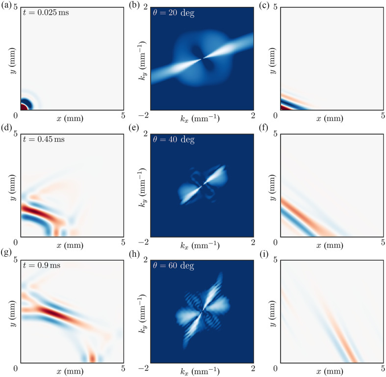
Approach: When a line source is used to launch plane mechanical waves over the medium surface, the phase velocity of Rayleigh waves in the direction of propagation is directly accessible. For a point-like source, propagation of the energy flux is tracked (i.e., its group velocity), which cannot be directly used for moduli inversion. In this case, angular spectrum decomposition is used to access the phase velocity. Both numerical simulations in OnScale and experiments in a stretched PVA phantom were performed.

Results: We show that both methods (line source wave excitation and angular decomposition from a point-like source) produce similar results and accurately estimate the angular anisotropy of the Rayleigh wave phase velocity. We also explicitly show that a commonly used group velocity approach leads to inadequate moduli inversion and should not be used for reconstruction.

Conclusions: We suggest that the line source is best when a surface area must be scanned, whereas the point-like source with the proposed phase velocity reconstruction is best for single-point moduli estimation or when tissue motion is a concern.

Keywords: Rayleigh waves; elastic moduli of soft tissues; group velocity; nearly-incompressible transverse isotropic; optical coherence elastography; phase velocity.

Fig. 1

Wavefields generated by a point-like source at different time moments from the excitation: (a) $t=0.025\text{ms}$, (b) $t=0.450\text{ms}$, and (c) $t=0.900\text{ms}$. For this case, $\mu =10\mathrm{kPa}$, $G/\mu =4$, $\delta /\mu =0$. Note, that $E_L$ and $E_T$ are the same for this case (i.e., there is no tensile anisotropy) (Video 1, MP4, 6.16 MB [URL: https://doi.org/10.1117/1.JBO.30.12.124503.s1]).

Fig. 2

Wavefields generated by a line source at different propagation directions characterized by angle $\theta$ relative to the symmetry axis $Z$ at different time moments from the excitation. For this particular case, $\mu =10\mathrm{kPa}$, $G/\mu =4$, $\delta /\mu =0$. Young’s moduli $E_L$ and $E_T$ are the same for this case (i.e., there is no tensile anisotropy). Panels (a)–(c): $\theta =0\mathrm{deg}$, time instants from the excitation are $t=0.025\text{ms}$, $t=0.45\text{ms}$, and $t=0.9\text{ms}$, respectively. Panels (d)–(f): $\theta =33\mathrm{deg}$, time instants from the excitation are $t=0.025\text{ms}$, $t=0.45\text{ms}$, and $t=0.9\text{ms}$, respectively. Panels (g)–(i): $\theta =45\mathrm{deg}$, time instants from the excitation are $t=0.025\text{ms}$, $t=0.45\text{ms}$ and $t=0.9\text{ms}$, respectively (Video 2, MP4, 6.11 MB [URL: https://doi.org/10.1117/1.JBO.30.12.124503.s2]).

Fig. 3

Comparison of Rayleigh wave velocities computed from numerically simulated (OnScale) wave propagation using a correlation method for both point-like and line sources of Rayleigh wave excitation. NITI medium mechanical moduli are the same as in Figs. 1 and 2: $\mu =10\mathrm{kPa}$, $G/\mu =4$, $\delta /\mu =0$ (significant shear anisotropy but no tensile anisotropy). (a) Comparison of the spatial signal profiles for point-like and line sources for two time moments ($t_1=0.4\mathrm{ms}$ and $t_2=0.9\mathrm{ms}$) in the direction of (a) $\theta =15\mathrm{deg}$ and (b) $\theta =75\mathrm{deg}$ relative to the symmetry axis. Comparison of the theoretically calculated group (dashed blue line) and phase (dashed red line) velocities and the measured Rayleigh wave speed using cross-correlation for point source (c) and line source (d) excitation. The colormap corresponds to the amplitude of the wave at $t=0.9\mathrm{ms}$, computed as the integral of the absolute value of the wavefields shown in (a) and (b) for every direction.

Fig. 4

Comparison of Rayleigh wave velocities computed from numerically simulated (OnScale) wave propagation using a correlation method for both point-like and line sources for a broad range of NITI medium mechanical properties: (a) $G/\mu =1$, $\delta /\mu =0$, (b) $G/\mu =1$, $\delta /\mu =2$, (c) $G/\mu =1$, $\delta /\mu =4$, (d) $G/\mu =2$, $\delta /\mu =0$, (e) $G/\mu =2$, $\delta /\mu =2$, (f) $G/\mu =2$ $\delta /\mu =4$, (g) $G/\mu =4$, $\delta /\mu =0$, (h) $G/\mu =4$, $\delta /\mu =2$, (i) $G/\mu =4$, $\delta /\mu =4$. Solid curves correspond to ground truth values of phase (red curve) and group (blue curve) velocities of Rayleigh waves computed analytically.

Fig. 5

Angular decomposition method to compute the phase velocity of Rayleigh waves launched by a point-like source in a NITI medium. NITI medium mechanical moduli are the same as in Figs. 1 and 2: $\mu =10\mathrm{kPa}$, $G/\mu =4$, $\delta /\mu =0$ (i.e., significant shear anisotropy but no tensile anisotropy). (a), (d), (g) Wavefields originating from the point-like source at different time instants as indicated in the top left corner of the panels. (b), (e), (h) 2D spatial spectra computed for the wavefields (a), (d), (g) respectively and their filtration with a 5 deg width Gaussian angular filter in the propagation direction indicated in the top left corner of each spectral panel. (c), (f), (i) – filtered waveforms for the same time instants (a), (d), (g) and directions (b), (e), (h).

Fig. 6

Rayleigh wave phase velocity angular dependence (blue dotted curve) obtained by spatial filtration (described in Sec. 4.1.2) of wavefields originating from the point-like source for a broad range of NITI medium mechanical properties: (a) $G/\mu =1$, $\delta /\mu =0$, (b) $G/\mu =1$, $\delta /\mu =2$, (c) $G/\mu =1$, $\delta /\mu =4$, (d) $G/\mu =2$, $\delta /\mu =0$, (e) $G/\mu =2$, $\delta /\mu =2$, (f) $G/\mu =2$, $\delta /\mu =4$, (g) $G/\mu =4$, $\delta /\mu =0$, (h) $G/\mu =4$, $\delta /\mu =2$, (i) $G/\mu =4$, $\delta /\mu =4$. Results are compared with phase velocity angular dependences computed directly using wavefields originating from a line source (blue dotted curve). Theoretically predicted (i.e. ground truth values) phase (solid red curve) and group (solid blue curve) velocity angular distributions are plotted for comparison.

Fig. 7

Dynamic OCE measurements with a line A μT source of Rayleigh waves in the anisotropic (NITI) PVA phantom. (a)–(c) Distance-time (XT) plots for different propagation directions: 0, 40, and 90 deg, respectively. Overall, XT plots were recorded for 19 propagation directions (every 10 deg) between forward and backward propagation. (d) Rayleigh-wave angular anisotropy computed using XT plots and reconstructed mechanical moduli of the phantom. The red curve in panel (d) corresponds to fitting experimental data with the NITI model (open circles). The black line in panel (d) corresponds to error bars, computed from the standard deviation over three repeated scans at each location (Video 3, MP4, 9.43 MB [URL: https://doi.org/10.1117/1.JBO.30.12.124503.s3]).

References

1. Leartprapun N., Adie S. G., “Recent advances in optical elastography and emerging opportunities in the basic sciences and translational medicine,” Biomed. Opt. Express 14(1), 208–248 (2022). 10.1364/BOE.468932 - DOI - PMC - PubMed
1. Zvietcovich F., Larin K. V., “Wave-based optical coherence elastography: the 10-year perspective,” Prog. Biomed. Eng. 4(1), 012007 (2022). 10.1088/2516-1091/ac4512 - DOI - PMC - PubMed
1. Zaitsev V. Y., et al. , “Strain and elasticity imaging in compression optical coherence elastography: the two-decade perspective and recent advances,” J. Biophotonics 14(2), e202000257 (2021). 10.1002/jbio.202000257 - DOI - PubMed
1. Kirby M. A., et al. , “Optical coherence elastography in ophthalmology,” J. Biomed. Opt. 22(12), 121720 (2017). 10.1117/1.JBO.22.12.121720 - DOI - PMC - PubMed
1. Ambroziński Ł., et al. , “Acoustic micro-tapping for non-contact 4D imaging of tissue elasticity,” Sci. Rep. 6, 38967 (2016). 10.1038/srep38967 - DOI - PMC - PubMed