Identification of rare cortical folding patterns using unsupervised deep learning

Abstract

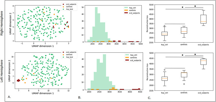
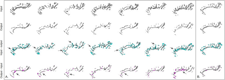
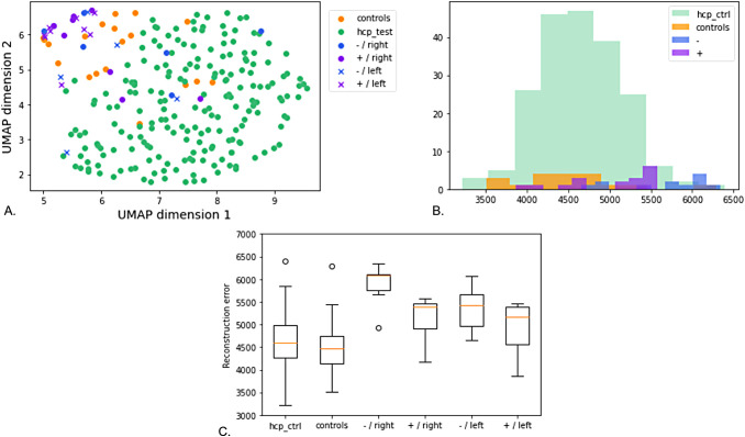
Like fingerprints, cortical folding patterns are unique to each brain even though they follow a general species-specific organization. Some folding patterns have been linked with neurodevelopmental disorders. However, due to the high inter-individual variability, the identification of rare folding patterns that could become biomarkers remains a very complex task. This paper proposes a novel unsupervised deep learning approach to identify rare folding patterns and assess the degree of deviations that can be detected. To this end, we preprocess the brain MR images to focus the learning on the folding morphology and train a beta variational auto-encoder ( $\beta -VAE$ ) on the inter-individual variability of the folding to identify outliers. We compare the detection power of the latent space and of the reconstruction errors, using synthetic benchmarks and one actual rare configuration related to the central sulcus. Finally, we assess the generalization of our method on a developmental anomaly located in another region and we validate the relevance of our approach on patients suffering from drug-resistant epilepsy. Our results suggest that this method enables encoding relevant folding characteristics that can be enlightened and better interpreted based on the generative power of the $\beta -VAE$ . The latent space and the reconstruction errors bring complementary information and enable the identification of rare patterns of different nature. This method generalizes well to a different region on another dataset and demonstrates promising results on the epileptic patients. Code is available at https://github.com/neurospin-projects/2022_lguillon_rare_folding_detection.

Keywords: Folding patterns; anomaly detection; cortical folding; cortical sulci; epilepsy; unsupervised learning; β − VAE.

Fig. 1.

Central sulcus region variability. (A) Localization of the studied region of interest (ROI) on a 3D view of one right hemisphere. The colored ribbons represent sulci, defined as a negative cast of the furrows. The central sulcus is red. (B) Examples of non-interrupted central sulci. (C) Examples of interrupted central sulci.

Fig. 2.

Overview of the BrainVISA/Morphologist pipeline’s main steps and of the folds representation. (A) Main steps of BrainVISA/Morphologist pipeline. 1. Raw T1-w MRI, 2. Bias-corrected image, 3. Segmentation of the brain, 4. Segmentation of the hemispheres and of the grey and white matter, 5. Skeleton representation of the folding graph, representing a negative cast of the 4. 6. Mesh representation of the white matter of the right hemisphere, 7. Folding graph that represents the folds (in green) as the negative cast of the white matter of the right hemisphere (white mesh).(B) Folds representation. 1. Example of a central sulcus, which is composed of several elementary entities called simple surfaces (SS). (Orientation: A: Anterior, P: Posterior, S: Superior, I: Inferior). 2. Corresponding schematic representation of the sulcus represented in 1, which is formed by four simple surfaces. Depth variation caused by the buried gyrus and the presence of two branches lead to the division into four different simple surfaces. 3. Corresponding folding graph.

Fig. 3.

Pipeline. A mask of the central sulcus area is defined based on a distinct manually labeled dataset. HCP is processed with Morphologist to obtain folding graphs, which are used to obtain 3D images of skeletons (1). The Chamfer distance is applied to the skeletons to obtain geodesic distance maps (2). Distance maps are then downsampled, registered to the ICBMc2009 space, cropped according to the mask (3), and fed as input to a $\beta -VAE$. Labeled sulci are only used to define the masks once, before any preprocessing and training. Once the masks are defined on the external dataset, no labels are used to model inter-individual variability and identify outliers.

Fig. 4.

Deletion benchmarks. Visualization of original sulcal pattern and its altered versions from the four deletion benchmarks showing patterns with increasing simple surface size deleted. Upper row: Mesh visualization. Middle and bottom rows: distance maps on axial view, visualization at depths 15 and 37.

Fig. 5.

Asymmetry benchmark. Visualization of the original sulcal pattern and its flipped contralateral version for two subjects.

Fig. 6.

Deletion benchmarks results. For each row, controls are represented in green and benchmark data in pink. Left column: UMAP projection of benchmark and control data. Middle column: ROC curves of classification of control and benchmark data. Right column: reconstruction error distributions and p-value of the Kolmogorov-Smirnov test with the null hypothesis that the two samples come from the same distribution.

Fig. 7.

Asymmetry benchmark results. Controls are represented in green and benchmark data in blue. (A) UMAP projection of benchmark and control data, ROC curves of classification of control and benchmark data, and reconstruction error distributions. (B) Averages for the control subjects, that is, right hemispheres (in green), and for the highlighted asymmetry subjects, that is, left hemispheres (in blue). These averages are also placed on the UMAP dimensions. (C) 1. and 2. Respectively side and bottom views of the averages of B. The single star indicates a single-knob configuration, and the two stars indicate the second knob of a double-knob configuration. (C) 3. Superposition of the two averages respectively in upper and bottom view.

Fig. 8.

Interrupted central sulci on UMAP space. (A) Interrupted central sulci shape distribution in the UMAP space. The 3D folding patterns of the subjects are positioned according to their location in the UMAP space. For instance, the pattern located in the lower left corner corresponds to subject 510225 in the UMAP representation. Subjects with interrupted sulci on the upper left of the UMAP visualization seem to correspond to an interruption with a T-shape pattern. (B) Outlier detection performances using OCSVM and isolation forest on the interrupted CS. (C) Controls and interrupted CS reconstruction error distributions.

Fig. 9.

Reconstructions and residuals for all seven interrupted sulci. (A) For all rows, distance maps are converted to meshes for an easier visualization. First row: input data. Second row: reconstruction of the model. Third row: Reconstruction of the model with the difference between the input and the output, that is, the model’s omissions (in blue). The purple arrow highlights an omission corresponding to a perpendicular branch pointing toward the frontal cortex. Last row: Reconstruction of the model with the difference between the output and the input, that is, the model’s additions (in purple). (B) Rotated view of the reconstructions represented with asterisks in the last row of A. The asterisks show interruptions of the central sulcus which have been filled by the model.

Fig. 10.

Results on corpus callosum dysgenesis (CCD) subjects. First row: right hemisphere. Bottom row: left hemisphere. For both rows: (A) UMAP projections of CCD subjects, control children, and HCP test. (B) Reconstruction error distributions for the CCD subjects, control children, and HCP test. (C) Reconstruction error variations for the CCD subjects, control children, and HCP test. Significant differences between populations according to the Mann-Whitney test are indicated with an asterisk.

Fig. 11.

Right cingulate sulcus reconstructions and residuals for the CCD subjects and one control. (A) CCD subjects. (B) One control subject from the same cohort. For both (A) and (B): each column corresponds to a subject. For all rows, distance maps are converted to meshes for an easier visualization. First row: input data. Second row: reconstruction of the model. Third row: Reconstructions of the model with the difference between the input and the output, that is, the model’s omissions. Last row: Reconstructions of the model with the difference between the output and the input, that is, the model’s additions. The arrows highlight interesting features added or missed by the model.

Fig. 12.

Results on patients suffering from FCD2. (A) UMAP projection of patients with a positive MRI (indigo), patients with a negative MRI (blue), controls of the same dataset (orange), and HCP test subjects (green). The crosses correspond to subjects with a lesion in the left hemisphere. (B) Reconstruction error distributions for the four groups (patients with negative or positive MRI, controls, and HCP subjects). (C) Reconstruction error variations for the different groups. Patients of each group have been separated depending on the lesion’s location.

Fig. 13.

Traveling through the latent space from the control centroid to the centroid of each group of patients and beyond. The insets are the centroid-generated patterns. We travel through the latent space from the control centroid to each patient group centroid and beyond as illustrated by the arrows. The intermediate patterns between the insets correspond to interpolations along the arrows. First row: From controls to +/right patients. Second row: From controls to -/right patients. Only patients with lesions located in the right hemisphere were used to generate the averages. Colors match Figure 12: controls are represented in orange, patients with positive MRI in indigo, and patients with negative MRI in blue.

Fig. 14.

Right central region reconstructions and residuals for the patients suffering from FCD2 and controls. Each column corresponds to a subject from each group (control, patient with a positive MRI, patient with a negative MRI). For all rows, distance maps are converted to meshes for easier visualization. First row: input data. Second row: reconstruction of the model. Third row: Reconstructions of the model with the difference between the input and the output, that is, the model’s omissions. Note that all patients represented have the lesion located in the right hemisphere.

References

1. Auzias, G., Brun, L., Deruelle, C., & Coulon, O. (2015). Deep sulcal landmarks: Algorithmic and conceptual improvements in the definition and extraction of sulcal pits. NeuroImage, 111, 12–25. 10.1016/j.neuroimage.2015.02.008 - DOI - PubMed
1. Auzias, G., Viellard, M., Takerkart, S., Villeneuve, N., Poinso, F., Fonséca, D. D., Girard, N., & Deruelle, C. (2014). Atypical sulcal anatomy in young children with autism spectrum disorder. NeuroImage: Clinical, 4, 593–603. 10.1016/j.nicl.2014.03.008 - DOI - PMC - PubMed
1. Baur, C., Denner, S., Wiestler, B., Albarqouni, S., & Navab, N. (2020). Autoencoders for unsupervised anomaly segmentation in brain MR images: A comparative study. arXiv:2004.03271 [cs, eess] http://arxiv.org/abs/2004.03271 - PubMed
1. Behrendt, F., Bengs, M., Rogge, F., Krüger, J., Opfer, R., & Schlaefer, A. (2022). Unsupervised anomaly detection in 3D brain MRI using deep learning with impured training data. In 2022 IEEE 19th International Symposium on Biomedical Imaging (ISBI) (pp. 1–4). 10.1109/isbi52829.2022.9761443 - DOI
1. Bénézit, A., Hertz-Pannier, L., Dehaene-Lambertz, G., Monzalvo, K., Germanaud, D., Duclap, D., Guevara, P., Mangin, J. F., Poupon, C., Moutard, M.L., & Dubois, J. (2015). Organising white matter in a brain without corpus callosum fibres. Cortex, 63, 155–171. 10.1016/j.cortex.2014.08.022 - DOI - PubMed
LinkOut - more resources