. 2025 Jul 30:16:1576686.
doi: 10.3389/fmicb.2025.1576686. eCollection 2025.

Transcutaneous auricular vagus nerve stimulation regulates gut microbiota mediated peripheral inflammation and metabolic disorders to suppress depressive-like behaviors in CUMS rats

Affiliations

Transcutaneous auricular vagus nerve stimulation regulates gut microbiota mediated peripheral inflammation and metabolic disorders to suppress depressive-like behaviors in CUMS rats

Xinjiang Zhang et al. Front Microbiol. .

Abstract

Background: Depression is a common mental disorder, and the changes of intestinal microflora and peripheral plasma metabolites can affect the gut-brain axis through vagus nerve, leading to the occurrence, and progress of the disease. Transcutaneous auricular vagus nerve stimulation (taVNS) has been previously shown to be clinically safe and effective in treating depression. However, there is no evidence whether its antidepressant effect is related to the regulation of intestinal flora and metabolites.

Objective: This study investigated the gut microbiota and plasma metabolism mechanisms of taVNS in the treatment of depression.

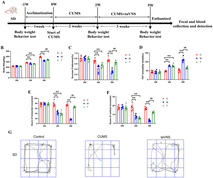
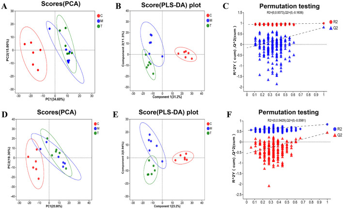
Methods: In this study, we established a chronic unpredictable mild stress (CUMS) model in SD rats for 5 weeks. During the last 3 weeks of CUMS treatment, the rats received continuous taVNS intervention for 3 weeks. Depressive-like behavior in SD rats was evaluated through behavioral assessments. The gut microbiota and plasma were analyzed using 16S rRNA gene sequencing and liquid chromatography-mass spectrometry (LC-MS) techniques.

Results: Behavioral tests showed that taVNS significantly reversed the depressive-like behavior induced by CUMS in rats. 16S rRNA sequencing results showed that taVNS could improve the intestinal flora structure of CUMS rats. Microbial community characterization index showed that taVNS could reverse the gut microbiota dysbiosis in CUMS rats. ROC analysis revealed that Lachnospiraceae_NK4A136_group. Parabacteroides and Corynebacterium_1 are potential biomarkers for diagnosing gut microbiota dysbiosis in CUMS rats and could also serve as potential therapeutic targets for taVNS. Plasma metabolomics results showed that the differential metabolites between the CUMS group and the control group were primarily enriched in pathways such as bile acid metabolism, arachidonic acid metabolism and ether lipid metabolism. The differential metabolites between the taVNS group and the CUMS group were primarily enriched in pathways related to vitamin digestion and absorption, glycerophospholipid metabolism and amino acid metabolism. Correlation analysis between the gut microbiota and plasma metabolites suggested that pathogenic microbial genera such as Lachnospiraceae, Lactobacillus, and Tyzzerella were positively correlated with plasma metabolites during inflammation, bile acid, and lipid metabolism dysregulation, while beneficial microbiota showed the opposite trend.

Conclusion: This study demonstrated that taVNS can regulate the gut microbiota, including Lachnospiraceae, Lactobacillus, Tyzzerella, and Bacteroides genera, which mediate peripheral inflammation, bile acid, and lipid metabolism dysregulation, thereby reversing the depressive-like behavior induced by CUMS in rats and exerting an antidepressant effect.

Keywords: brain-gut axis; depression; gut microbiota; metabolomics; transcutaneous auricular vagus nerve stimulation.


Conflict of interest statement

The authors declare that the research was conducted in the absence of any commercial or financial relationships that could be construed as a potential conflict of interest.

Figures

Illustration of a mouse connected to an electrotherapy device labeled HANS-200A, displaying settings of 2/15 Hz, 2 mA, and 30 min. An electrode is shown inserted into auricular nail cavities of rats, indicating a medical procedure or experiment.
Figure 1
The diagram of transcutaneous auricular vagus nerve stimulation. The electrical stimulation was applied to the auricular branch of the vagus nerve distribution area, as indicated in the enlarged part of the above figure.
Research diagram showing an experimental timeline, data charts, and movement paths. Panel A depicts a five-week timeline from acclimatization to euthanization with phases for CUMS and taVNS treatments. Panels B–F show bar graphs comparing body weight, sucrose preference, FST immobility time, and movement scores across control (C), model (M), and treatment (T) groups at different weeks. Panel G displays movement paths for control, CUMS, and taVNS groups in an open field test. Statistically significant differences are indicated with asterisks and hashes.
Figure 2
Effects of taVNS on body weight and depressive-like behaviors in CUMS rats (n = 6). (A) Schematic diagram of CUMS model establishment and schematic diagram of taVNS intervention. (B) Comparison of body weight at different time points. (C) Sucrose preference rate at different time points. (D) Comparison of immobility time of forced swimming at different time points. (E) Comparison of horizontal motion scores at different time points. (F) Comparison of vertical motion scores at different time points. (G) Representative activity traces of subjects in different groups for SD rats in the open field test. Significant group effects were observed for body weight (F = 92.6), sucrose preference test (F = 38.35), forced swimming test (F = 63.97), horizontal movement distances (F = 126.4), and vertical movement distances (F = 67.62). Compared with control group, **p < 0.01; Compared with CUMS group, ##p < 0.01. C, Control group; M, Model group (CUMS group); T, Intervention group (taVNS group).
Five graphs depict diversity measures. Graph A shows Shannon curves depicting diversity across read samples for groups C, M, T. Graph B illustrates rarefaction curves for the same groups, assessing observed species richness. Graph C presents a box plot of the Sobs index at the OTU level with p = 0.54. Graph D shows a box plot for the Chao index with p = 0.2199. Graph E displays a box plot for the Shannon index with p = 0.5287. Legends identify groups C, M, T in red, blue, and green.
Figure 3
Alpha diversity of intestinal microbial samples of rats in each group (n = 6). (A, B) OTU sparse Shannon index curve and dilution curve of samples. (C) Sobs index. (D) Chao index. (E) Shannon index. C, Control group; M, Model group (CUMS group); T, Intervention group (taVNS group).
Panel A shows a PCoA plot on OTU levels with ellipses for groups C, M, and T, indicating clustering. Panel B displays a PLS-DA plot showing separation of groups based on components. Panel C features a box plot comparing beta diversity among groups C, M, and T, with statistical significance indicated by a Kruskal-Wallis test (p = 0.001779). Panel D shows a box plot comparing beta diversity between groups C and M using a Student's t-test (p = 0.04665). Panel E illustrates a box plot comparison for groups M and T, with significant differences (p = 7.874e-05) using a Student's t-test.
Figure 4
Beta diversity of intestinal microbial samples of rats in each group (n = 6). (A) PCoA analysis. (B) PLS-DA analysis. (C–E) Beta diversity difference analysis between groups. C, Control group; M, Model group (CUMS group); T, Intervention group (taVNS group).
Violin plots (A–C) display GMHI and MDI indices across groups C, M, and T with statistical significance indicated. A Venn diagram (D) shows overlaps in data sets, with a bar plot below displaying quantities for each group. Bar plots (E–H) illustrate sample counts and relative abundances for various microbial groups across the three conditions. Circos plots (I–J) depict complex relationships and interactions between microbial taxa, highlighting connections and relative abundances within groups C, M, and T.
Figure 5
Analysis of microbial community characterization index and composition ratio (n = 6). (A–C) analysis of GMHI and MDI index; (D) analysis of flora in each group by Venn diagram; (E, F) analysis of flora typing in each group by phylum and genus level; (G, H) analysis of colony composition in each group by Bar diagram. (I, J) Circos samples and species relationship analysis of each group at phylum and genus level. C, Control group; M, Model group (CUMS group); T, Intervention group (taVNS group).
Three-part image analyzing microbial data. A: A circular phylogenetic tree with colored branches and labels denoting different microbial taxa, with red, blue, and green indicating groups C, M, and T. B: A bar chart showing LDA scores for various taxa, with red, blue, and green bars representing groups C, M, and T. C: A bar chart displaying mean proportions of different taxa, with bars colored red, blue, and green for groups C, M, and T, respectively.
Figure 6
Multilevel discriminant analysis of Lefse species difference and inter-group difference test for each group (n = 6). (A, B) Branch and bar graphs generated by LEfSe analysis showed different classification levels among each group (LDA > 3.0). (C) Kruskal-Wallis rank sum test for the differential flora between groups. The Y-axis represents the species name, the X-axis represents the average relative abundance in different groups of species, and the far right is the P-value. C, Control group; M, Model group (CUMS group); T, Intervention group (taVNS group).
Panel A shows a bar chart comparing proportions of bacterial groups between two categories, C and M, with confidence intervals, p-values, and effect sizes. Panels B, C, and D display ROC curves with sensitivity and specificity, each having an AUC of 0.97, 0.93, and 0.94 respectively, representing high discriminatory power.
Figure 7
Differential flora test and ROC analysis (n = 6). (A) The T-test of the differential flora between the CUMS group and the blank control group formed a bar chart, in which the Y-axis represented the species name, the X-axis represented the average relative abundance of species in different groups, and the far right was the P-value. (B–D) Area under ROC curve of Lachnospiraceae_NK4A136_group, Parabacteroides, and Corynebacterium_1. X-axis was 1-Specificity, coordinate axis was 1–0; the Y-axis is Sensitivity and the coordinate axis is 0–1; the point marked on the curve is the optimal critical value. The AUC indicated in the figure is the area under the corresponding curve. C, blank control group; M, model group (CUMS group).
Panel A and D show PCA score plots with three groups: C (red), M (blue), T (green), indicating data separation. Panels B and E display PLS-DA plots with similar group separations. Panels C and F present permutation testing results, showing R2 and Q2 values over iterations, with R2 in blue and Q2 in red.
Figure 8
PCA and PLS-DA analysis of plasma metabolic samples from rats in each group (n = 6). (A–C) PCA and PLS-DA analysis plots in the negative ion mode. (D–F) PCA and PLS-DA analysis plots in the positive ion mode. C, Blank control group; M, Model group (CUMS group); T, Intervention group (taVNS group).
Graphical representation of metabolomic data analysis. Panel A shows a volcano plot highlighting significant metabolites. Panel B presents a KEGG enrichment analysis chart with rich factor values and p-values. Panels C to N contain bar graphs comparing the abundance of specific metabolites, such as Chenodeoxycholic Acid and L-Methionine, between control (C, red) and model (M, blue) groups. Statistical significance is indicated by asterisks above the bars.
Figure 9
Differential metabolites between groups and KEGG pathway enrichment analysis (n = 6). (A) Volcano plot of differential metabolites between the control group and the CUMS group. (B) KEGG pathway enrichment bubble plot of differential metabolites between the control group and the CUMS group. (C–N) Bar plots of t-test results for differential metabolites between the control group and the CUMS group (n = 6). Compared with the control group, *p < 0.05, **p < 0.01. C, Control group; M, Model group (CUMS group).
Composite image with multiple charts showing metabolomic data analysis: A) Volcano plot highlighting significant metabolites. B) KEGG enrichment analysis scatter plot, indicating overrepresented metabolic pathways with varying P-values. C–O) Bar graphs comparing the abundance of specific metabolites in two groups (M, T), with statistical significance denoted by asterisks or “ns” for not significant. Graphs illustrate differences in metabolite levels and pathway associations.
Figure 10
Differential metabolites between groups and KEGG pathway enrichment analysis (n = 6). (A) Volcano plot of differential metabolites between the CUMS group and the taVNS group. (B) KEGG pathway enrichment bubble plot of differential metabolites between the CUMS group and the taVNS group. (C–N) Bar plots of t-test results for differential metabolites between the control group and the CUMS group (n = 6). Compared with the CUMS group, *p < 0.05, **p < 0.01. ns, non-significant; M, Model group (CUMS group); T, Intervention group (taVNS group).
Heatmap depicting clustered data, displaying a range of metabolite interactions with bacterial genera. Rows represent metabolites, and columns represent bacterial genera, color-coded from red (positive correlation) to blue (negative correlation). Dendrograms on both axes illustrate hierarchical clustering.
Figure 11
Correlation analysis between gut microbiota and plasma metabolites. The right side of the figure shows the names of plasma metabolites, and the bottom lists the names of the gut microbiota. Each cell in the figure represents the correlation between two attributes (gut microbiota and plasma metabolites), with different colors indicating the strength of the correlation coefficient between the attributes. *P < 0.05, **P < 0.01, ***P < 0.001.

Similar articles

References

    1. Antoniuk S., Bijata M., Ponimaskin E., Wlodarczyk J. (2019). Chronic unpredictable mild stress for modeling depression in rodents: meta-analysis of model reliability. Neurosci. Biobehav. Rev. 99, 101–116. 10.1016/j.neubiorev.2018.12.002 - DOI - PubMed
    1. Beurel E., Toups M., Nemeroff C. B. (2020). The bidirectional relationship of depression and inflammation: double trouble. Neuron 107, 234–256. 10.1016/j.neuron.2020.06.002 - DOI - PMC - PubMed
    1. Brash A. R. (2001). Arachidonic acid as a bioactive molecule. J. Clin. Investig. 107, 1339–1345. 10.1172/JCI13210 - DOI - PMC - PubMed
    1. Camilleri M. (2021). Human intestinal barrier: effects of stressors, diet, prebiotics, and probiotics. Clin. Trans. Gastroenterol. 12:e00308. 10.14309/ctg.0000000000000308 - DOI - PMC - PubMed
    1. Chen M., Wang L., Lou Y., Huang Z. (2024). Effects of chronic unpredictable mild stress on gut microbiota and fecal amino acid and short-chain fatty acid pathways in mice. Behav. Brain Res. 464:114930. 10.1016/j.bbr.2024.114930 - DOI - PubMed

LinkOut - more resources