Comparative transcriptomics analysis of the Oleidesulfovibrio alaskensis G20 biofilms grown on copper and polycarbonate surfaces

Abstract

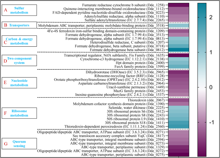
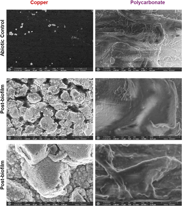
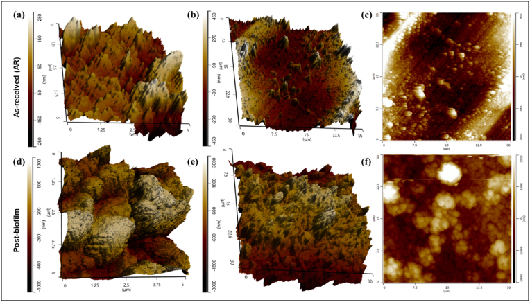
Sulfate-reducing bacterial (SRB) biofilms are prevalent across diverse environments, playing key roles in biogeochemical sulfur cycling while also contributing to industrial challenges such as biofouling and biocorrosion. Understanding the genetic and physiological adaptations of SRB biofilms to different surfaces is crucial for developing mitigation strategies. This study presents a comparative transcriptomic analysis of Oleidesulfovibrio alaskensis G20 biofilms grown on copper and polycarbonate surfaces, aimed at elucidating their differential responses at the molecular level. RNA sequencing revealed 1255 differentially expressed genes, with copper-grown biofilms exhibiting upregulation of Dde_1570 (flagellin; log2FC 2.31) and Dde_0831 (polysaccharide chain length determinant; log2FC 1.15), highlighting enhanced motility and extracellular polymeric substance production. Conversely, downregulated genes on copper included Dde_0132 (Cu/Zn efflux transporter; log2FC -3.37) and Dde_0369 (methyl-accepting chemotaxis protein; log2FC -1.19), indicating a metabolic shift and stress adaptation to metal exposure. Morphological analysis via SEM revealed denser biofilm clusters with precipitates on copper, whereas biofilms on polycarbonate were more dispersed. AFM analysis showed a 4.6-fold increase in roughness on copper (44.3 ± 3.1 to 205.89 ± 8.7 nm) and a 3.8-fold increase on polycarbonate (521.12 ± 15.2 to 1975.64 ± 52.6 nm), indicating surface erosion and structural modifications. Protein-protein interaction analysis identified tightly regulated clusters associated with ribosomal synthesis, folate metabolism, and quorum sensing, underscoring their role in biofilm resilience. Additionally, functional annotations of uncharacterized genes revealed potential biofilm regulators, such as Dde_4025 (cytochrome-like protein; log2FC 4.18) and Dde_3288 (DMT superfamily permease; log2FC 3.55). These findings provide mechanistic insights into surface-dependent biofilm formation, with implications for designing antifouling materials and controlling microbial-induced corrosion.

Keywords: Biocorrosion; Biofilm; Metallic; Non-metallic; SRB; Surface roughness; Transcriptomics.

Fig. 1

(A) Venn diagram of the total gene distribution and differentially expressed genes (DEGs) in the O. alaskensis G20 genome. The figure illustrates the entire set of genes in the O. alaskensis G20 genome as the superset. The subsets represent the total number of DEGs (0 ≤ p-value ≤1), DEGs with a p-value ≤0.05, and those with and without associated metabolic pathways. (B) The volcano plot displays the overall upregulated and downregulated DEGs with a p-value ≤0.05. The top 20 most significant genes are highlighted by their gene identifiers (Dde).

Fig. 2

The heatmap highlights the Rich Factor values across various pathways before and after filtering with the log2FC cutoff. Each column represents a distinct metabolic or biosynthesis pathway, with color intensity indicating the magnitude of the Rich Factor, where darker shades represent higher enrichment values. (For interpretation of the references to color in this figure legend, the reader is referred to the Web version of this article.)

Fig. 3

Gene frequency distribution across metabolic pathways, showing upregulated (green dots) and downregulated (purple crosses) genes. The top panel includes all DEGs (cyan bars), while the bottom panel shows DEGs filtered by cutoff (log2FC ≥ 1) (red bars). Pathways on the x-axis highlight variations in metabolic pathways, with the y-axis indicating gene frequency. (For interpretation of the references to color in this figure legend, the reader is referred to the Web version of this article.)

Fig. 4

The figure displays scatter plots representing z-scores for Gene Ontology (GO) terms associated with upregulated (Plot A) and downregulated (Plot B) genes derived from transcriptomics data. The x-axis of each plot shows the z-score, which quantifies the level of enrichment of each GO term, while the y-axis represents the -log10(p-value), indicating the statistical significance of the enrichment. Bubbles on the graph are sized according to the number of genes associated with each GO term, with larger bubbles representing terms with more genes. The colors denote different GO domains: cellular component (purple), molecular function (teal), and biological process (yellow). (For interpretation of the references to color in this figure legend, the reader is referred to the Web version of this article.)

Fig. 5

Protein-protein interaction (PPI) network showing DEGs clustered based on k-means clustering. The nodes are color-coded according to log2FC values, with the scale indicating the degree of gene upregulation (purple) and downregulation (teal green). (For interpretation of the references to color in this figure legend, the reader is referred to the Web version of this article.)

Fig. 6

The heatmap illustrates the differential gene expression across seven major functional categories. The data is presented using a gradient color scheme, where blue indicates upregulation and purple signifies downregulation. (For interpretation of the references to color in this figure legend, the reader is referred to the Web version of this article.)

Fig. 7

SEM images highlighting the As-Received (AR) surface of (a) polycarbonate, and (b) copper. Biofilm formation on (c, e, g) polycarbonates, and (d, f, h) copper surface on the 5th day.

Fig. 8

Quantification of total EPS (A) and its biochemical components (B) from O. alaskensis G20 biofilms grown on copper and polycarbonate surfaces at day 7.

Fig. 9

SEM images of O. alaskensis G20 biofilms formed on copper surfaces at day 7, highlighting morphological differences between nanowire-like structures (NW, yellow boxes) and pili (P, red boxes). Nanowires appear as long, thick, bundled filaments, often extending across cells and the substrate, while pili are thinner, shorter, and localized near individual cells. (For interpretation of the references to color in this figure legend, the reader is referred to the Web version of this article.)

Fig. 10

SEM images of copper (left) and polycarbonate (right) surfaces of abiotic control and after biofilm removal.

Fig. 11

Comparison of surface metrics (roughness, skewness, and kurtosis). The coral red and golden bars show the surface metrics for 5x5 and 30 × 30 μm², respectively. Standard deviations are represented by error bars. (For interpretation of the references to color in this figure legend, the reader is referred to the Web version of this article.)

Fig. 12

Topographical analysis of polycarbonate surfaces. (a, b) AR surface with 3D topographical views of areas 5 × 5 μm² and 30 × 30 μm², respectively. (c) Height map of the as-received surface (30 × 30 μm²). (d, e) PB surface with 3D topographical views of areas 5 × 5 μm² and 30 × 30 μm², respectively. (f) Height map of the post-biofilm surface (30 × 30 μm²).

Fig. 13

Topographical analysis of copper surfaces. (a, b) As-received surface with 3D topographical views of areas 5 × 5 μm² and 30 × 30 μm², respectively. (c) Height map of the as-received surface (30 × 30 μm²). (d, e) Post-biofilm surface with 3D topographical views of areas 5 × 5 μm² and 30 × 30 μm², respectively. (f) Height map of the post-biofilm surface (30 × 30 μm²).

References

-
- Krishnan S., Patil S.A., Nancharaiah Y. Material-microbes interactions. Elsevier; 2023. Environmental microbial biofilms: formation, characteristics, and biotechnological applications; pp. 3–45.
- Shineh G., et al. Biofilm formation, and related impacts on healthcare, food processing and packaging, industrial manufacturing, marine industries, and sanitation–a review. Appl Microbiol. 2023;3(3):629–665.
- Tuck B., et al. A critical review of marine biofilms on metallic materials. npj Mater Degrad. 2022;6(1):25.
LinkOut - more resources
Full Text Sources
Miscellaneous