A compressed hierarchy for visual form processing in the tree shrew

Abstract

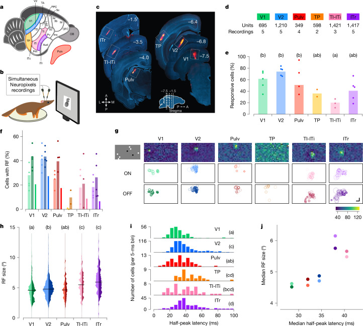
Our knowledge of the brain processes that govern vision is largely derived from studying primates, whose hierarchically organized visual system¹ inspired the architecture of deep neural networks². This raises questions about the universality of such hierarchical structures. Here we examined the large-scale functional organization for vision in one of the closest living relatives to primates, the tree shrew. We performed Neuropixels recordings^3,4 across many cortical and thalamic areas spanning the tree shrew ventral visual system while presenting a large battery of visual stimuli in awake tree shrews. We found that receptive field size, response latency and selectivity for naturalistic textures, compared with spectrally matched noise⁵, all increased moving anteriorly along the tree shrew visual pathway, consistent with a primate-like hierarchical organization^6,7. However, tree shrew area V2 already harboured a high-level representation of complex objects. First, V2 encoded a complete representation of a high-level object space⁸. Second, V2 activity supported the most accurate object decoding and reconstruction among all tree shrew visual areas. In fact, object decoding accuracy from tree shrew V2 was comparable to that in macaque posterior IT and substantially higher than that in macaque V2. Finally, starting in V2, we found strongly face-selective cells resembling those reported in macaque inferotemporal cortex⁹. Overall, these findings show how core computational principles of visual form processing found in primates are conserved, yet hierarchically compressed, in a small but highly visual mammal.

Fig. 1. High-throughput electrophysiological recordings along the tree shrew ventral visual pathway reveal a functional hierarchy.

a,b, Schematic of a tree shrew brain (a) and head-fixed electrophysiological recordings with Neuropixels probes (b). c, Representative electrode tracks marked with DiI (red) in each targeted area. Numbers indicate rostrocaudal position relative to Bregma (inset). A, anterior; L, lateral; M, medial; P, posterior. d, Number of recordings and total units across each area. e, Percentage of visually responsive cells to any of the presented visual stimuli in each area (Methods). Dots indicate individual recordings, bars indicate averages across recordings. Letters in this and subsequent panels indicate Tukey grouping. Tukey analysis (α = 0.05) after ANOVA, F_5,18 = 5.362, P = 0.003). f, Percentage of visually responsive units (see Fig. 1e) showing receptive fields (RFs). Left (lighter, ON), centre (darker, OFF) and right (ON/OFF) bars for each area. Dots indicate individual recording sessions. g, Distribution of receptive field locations across the visual field. Top row, receptive field maps for example units, one per area. Middle and bottom rows show the position and sizes of all ON and OFF receptive fields (respectively) in a representative recording. Shading indicates receptive field quality (Methods). Each white box represents ±54° horizontally and ±38° vertically. Top left, one frame of sparse noise stimulus used to map receptive fields. h, Distribution of ON (left, lighter) and OFF (right, darker) receptive field sizes for each area. Tukey analysis (α = 0.05) after ANOVA, F_4,1540 = 36.544, P < 10⁻²⁸; TP was excluded from this analysis because of the very low number of cells with receptive fields in this area. i, Histogram of the latencies to half-peak response in visually responsive cells in each area. Tukey analysis (α = 0.05) after ANOVA F_5,1147 = 20.197, P < 10⁻¹⁸. j, Comparison of the hierarchy inferred from receptive field size (y axis) and response latency (x axis). Each dot represents the median of the data for a given area (hue), with ON and OFF receptive fields represented by light and dark dots, respectively. Scale bar, 15°.

Fig. 2. Encoding of orientation, spatial frequency, and texture across tree shrew ventral visual areas.

a, Example frames of static grating stimuli. Stimuli were varied in orientation, spatial frequency and phase, and were interleaved with grey frames. b, Percentage of visually responsive cells (see Fig. 1e) that responded to static gratings in individual recording sessions (dots) and averaged across recording sessions (bars). c, Responses of a representative V2 and ITr cell to static gratings differing in orientation (represented circumferentially), spatial frequency (represented radially, cycles per degree) and phase (four small quadrants). Each dot represents a single trial; colour intensity represents responses strength. d, Percentage of variance of individual cells’ responses explained by orientation of the stimulus. Boxes represent 25th, 50th and 75th percentile; whiskers 5th and 95th. Letters in this and subsequent panels indicate Tukey grouping. Tukey analysis (α = 0.05) after ANOVA, F_5, 1106 = 26.791, P < 10⁻²⁴. Number of cells: V1 186, V2 500, Pulv 68, TP 79, TI-ITi 51 and ITr 228. e, Same for spatial frequency. Tukey analysis (α = 0.05) after ANOVA, F_5, 1106 = 20.514, P < 10⁻¹⁸ (same cells as d). f, Example frames of naturalistic texture (top) and spectrally matched noise (bottom). g, Percentage of visually responsive cells (see Fig. 1e) that responded to naturalistic texture or spectrally matched noise stimuli in individual recording sessions (dots) and averaged across recording sessions (bars). h, Time courses of population responses in each area to naturalistic texture (darker lines) and spectrally matched noise (lighter lines). Black arrows indicate the latency at which the two curves first significantly differed from each other (two-tailed t-test, P < 0.01). Shaded areas are standard errors of averages across cells. i, Percentage of variance in neural activity explained by texture image family (15 classes, see Fig. 2f).

Fig. 3. Objects are encoded across tree shrew ventral visual areas through axis coding.

a, Spike raster plots for representative visually active cells from each of the areas in response to six groups of object stimuli, each optimal for one of the cells (stimuli shown on the left). Each dot represents an action potential in one of up to ten presentations of the stimulus; red line indicates stimulus onset. b, Percentage of visually responsive cells (see Fig. 1e) that responded to object stimuli in individual recording sessions (dots) and averaged across recording sessions (bars). c, Percentage of variance of neural responses explained in each area by object stimulus identity (left bars) and by low-level feature image indices (right bars). d, Schematic illustrating the processing of visual stimuli in layers of the artificial neural network AlexNet (top) and in areas of the tree shrew ventral visual pathway (bottom). e, Normalized neural responses to object images for 100 randomly selected cells in each of the six areas as a function of position of that image along the given neuron’s preferred axis in AlexNet FC6 space (object space). The x axis is rescaled so that the range [−1,1] covers 98% of the stimuli. Inset, preferred axis (green arrow, Methods) of a representative cell (area V2) in object space. The coordinate axes represent the three AlexNet principal components (PCs) that most align with the cell’s preferred axis. Each dot represents an image, colour coded by the strength of the cell’s response to that image (blue, low; red, high). f, Responses as a function of normalized position along each cell’s principal orthogonal axis, that is, the axis in object space orthogonal to the neuron’s preferred axis that captured the most variance in AlexNet activations (Methods). Scale bar, 50 ms. Object images in panel a used with permission from ref. , Springer Nature Limited.

Fig. 4. Neural representation of object stimuli in tree shrew ventral visual areas reveals optimal feature decoding in area V2.

a, Variance of the responses of a representative V2 cell explained by individual AlexNet layers. Blue line shows the explainable variance of the cell. b, Histograms of explained variance by different layers of AlexNet for responses of visually responsive cells (n = 602) in area V2. Blue triangles mark values for the cell from a. c, Normalized explained variance by AlexNet layers for each tree shrew visual area (Methods). d, Variance of encoded neural activity in different areas explained by individual AlexNet FC6 principal components (PCs) as a percentage of explainable variance in that area. e, Percentage of variance of AlexNet FC6 features that can be explained by decoding from the neural responses in different areas. f, Ten examples of original images presented to the tree shrew and the images reconstructed from V2, V1 and TI-ITi: that is, the closest images to the predicted responses from AlexNet FC6 from an auxiliary database of images that were not shown to the animal (Methods). g. Average decoding distance for each tree shrew visual area between AlexNet FC6 activations predicted from neural activity and actual activations for each image, normalized by theoretical best decoding distance (Methods). Tukey analysis (α = 0.05) after ANOVA, F_6,11144 = 151.248, P < 10⁻¹⁸⁴. Object images in panel f used from ref. , Springer Nature Limited.

Fig. 5. Single cells across the tree shrew ventral stream show selectivity for different sectors of object space including faces.

a, Projections of 1,593 object images onto object space (the first two principal components from AlexNet layer FC6) with images from several categories (faces, animals, fruits) indicated. b, Projections of the preferred axes of all cells onto object space. c, Raster plots of several representative face-selective cells (circled in b) responding to face and object stimuli. The ten most preferred images for each cell are shown to the left of each raster. Arrowheads mark responses to those images. Red lines show stimulus onset. d, Raster plots of three representative V2 cells (arrowheads in b) with preferred axes in quadrants I, II and IV. Twenty stimuli from each quadrant were randomly chosen to generate raster plots. Right, top five preferred images for each cell. e, Histograms of t scores for face selectivity across areas. Scale bars, 50 ms (c), 50 ms (d). Object images in panels c and d used from ref. , Springer Nature Limited.

Fig. 6. Comparison of object responses between primate and tree shrew ventral visual areas.

a, Schematic of recordings in primate. b, Simultaneous Neuropixels recordings from three nodes in macaque monkey cortex. Neuropixels NHP 1.0 probes were inserted into V2, posterior IT and anterior IT cortex. c, Responses of cells in V2, posterior IT and anterior IT, respectively (rows), to 96 stimuli composed of faces and objects (columns). Only visually responsive cells were included (two-tailed t-test, P < 0.05). d, Percentage of variance of neural responses explained by object stimulus identity in each area. e, Average decoding distance for each visual area between AlexNet FC6 activations predicted from neural activity and actual FC6 activations for each image, normalized by theoretical best decoding distance (Methods). f, Histograms of t-scores for face selectivity across areas. g, Decoding performance for individual object identity (dashed lines) or face identity (solid lines) as a function of number of cells used by the classifier. Note the overlap of the two lines for TI-ITi. Black lines indicate decoding performance for face identity using only face cells (t > 5). Dashed grey lines show chance level for object decoding. h, Schematic comparing macaque, tree shrew and rodent visual systems. Object images in panel c used from ref. , Springer Nature Limited.

Extended Data Fig. 1. Anatomical inputs to intermediate (TP) and anterior (ITr) nodes of the tree shrew ventral pathway.

(a) Schematic of injections of retrograde tracer CTβ−488 (green) into TP and CTβ-594 (red) into ITr. (b) Coronal histological sections showing retrogradely labeled cells projecting to TP (green) and ITr (red) and counterstained with DAPI (grey). Representative samples out of n = 2 animals. Scale bars: 1 mm / 0.5 mm (insets). Adapted with permission from ref. , Springer.

Extended Data Fig. 2. Object responses are largely not accounted by low-level features.

(a) Examples of the two images with the lowest (left) and highest (right) value for horizontality, internal contrast, circularity and area. (b) Histogram indicating the average fraction of variance in the firing rate explained by various low-level image feature indices. (c) Schematic of quantification of luminance and contrast impinging on each receptive field. We computed the average luminance and contrast (second derivative of luminance) falling inside the ON and OFF receptive fields of each cell, and average across the two. (d) Percentage of variance of neural responses explained by object stimulus identity in each area. Dark bars correspond to the part of the variance accounted for by luminance impinging each receptive field. (e) Same, but dark bars correspond to contrast. (f) Representative objects with increasing high spatial frequency content from low (leftmost column) to high (rightmost column). (g) Power spectrum across groups of images in (a) relative to the middle spatial frequency group. (h) Percentage of variance of neural responses explained by object stimulus identity in each area, separated into categories based on spatial frequency. Object images in panels a, c and f used from ref. , Springer Nature Limited.

Extended Data Fig. 3. Explanatory power of AlexNet and image reconstruction.

(a) Aggregate explanatory power of the AlexNet layer that best explained each given area. (b) Fraction of variance in the firing rates of individual cells (dots) explained by different AlexNet layers plotted against the fraction of the total explainable variance in that cell (Methods). (c) Aggregate explanatory power of AlexNet layer FC6 over different areas. (d) Schematic of image reconstruction approach. Images in panel d used from ref. , Springer Nature Limited.

Extended Data Fig. 4. Cells selective to different sectors of object space with no obvious topographical organization in object space for each area.

(a) Left: Projections of each TI-ITi cell’s preferred axis onto the first two PCs of object space (replicated from Fig. 5b). Right: Raster plots of three representative TI-ITi cells from quadrants I, II, and IV indicated by letters; twenty stimuli from each quadrant were randomly chosen to generate raster plots. Scale bar: 50 ms. Top five preferred images for each cell. (b) Same for ITr. (c) Selectivity of cells in each area as a function of recording depth along the Neuropixels probe. In each of the six plots, each dot represents one cell, the color of the dots indicates the depth at which the cell was recorded (inset, right), and the position of the dot indicates the mean projection of the 10 most preferred images onto the first two PCs of object space. Object images in panels a and b used from ref. , Springer Nature Limited.

Extended Data Fig. 5. DNN-predicted indices of view invariance are similar across all tree shrew ventral visual areas.

(a) Schematic showing workflow for predicting neuron responses for a new set of stimuli. 1593 images were passed through AlexNet (top). Activations in AlexNet layer FC6 were used to linearly predict neural responses evoked by each image when shown to the animal. This yields a weight matrix W that optimally predicts a neuron’s response based on the image features F. Next, the weight matrix is used to predict neuron responses to 1224 images consisting of 51 objects at 24 views that were not shown to the tree shrew (bottom). (b) Responses of three example cells from macaque V2, posterior IT and anterior IT, to 50 objects (columns) each at 24 different views (rows). Top panel show actual responses, bottom panel shows responses predicted from an AlexNet model built from responses to 1593 images (see Extended Data Fig. 5a). (c) Same as (b) but for predicted responses of six example tree shrew neurons from all areas. (d) Histograms of invariance indices (Methods) of macaque V2, posterior IT and anterior IT neurons, calculated from actual responses (left) and predicted responses (right). Vertical lines indicate means. (e) Histograms of invariance indices of predicted responses across all tree shrew areas. Object images in panel a used from ref. , Springer Nature Limited.

References

1. Felleman, D. J. & Van Essen, D. C. Distributed hierarchical processing in the primate cerebral cortex. Cereb. Cortex1, 1–47 (1991). - PubMed
1. LeCun, Y., Bengio, Y. & Hinton, G. Deep learning. Nature521, 436–444 (2015). - PubMed
1. Jun, J. J. et al. Fully integrated silicon probes for high-density recording of neural activity. Nature551, 232–236 (2017). - PMC - PubMed
1. Trautmann, E. M. et al. Large-scale high-density brain-wide neural recording in nonhuman primates. Nat. Neurosci.28, 1562–1575 (2025). - PMC - PubMed
1. Freeman, J., Ziemba, C. M., Heeger, D. J., Simoncelli, E. P. & Movshon, J. A. A functional and perceptual signature of the second visual area in primates. Nat. Neurosci.16, 974–981 (2013). - PMC - PubMed
LinkOut - more resources