Brain-wide representations of prior information in mouse decision-making

Abstract

The neural representations of prior information about the state of the world are poorly understood¹. Here, to investigate them, we examined brain-wide Neuropixels recordings and widefield calcium imaging collected by the International Brain Laboratory. Mice were trained to indicate the location of a visual grating stimulus, which appeared on the left or right with a prior probability alternating between 0.2 and 0.8 in blocks of variable length. We found that mice estimate this prior probability and thereby improve their decision accuracy. Furthermore, we report that this subjective prior is encoded in at least 20% to 30% of brain regions that, notably, span all levels of processing, from early sensory areas (the lateral geniculate nucleus and primary visual cortex) to motor regions (secondary and primary motor cortex and gigantocellular reticular nucleus) and high-level cortical regions (the dorsal anterior cingulate area and ventrolateral orbitofrontal cortex). This widespread representation of the prior is consistent with a neural model of Bayesian inference involving loops between areas, as opposed to a model in which the prior is incorporated only in decision-making areas. This study offers a brain-wide perspective on prior encoding at cellular resolution, underscoring the importance of using large-scale recordings on a single standardized task.

Fig. 1. Mice use the block prior to improve performance.

a, Mice had to move a 35° peripheral visual grating to the centre of the screen by turning a wheel with their front paws. The contrast of the visual stimulus varied from trial to trial. Adapted from ref. , eLife, under a CC BY 4.0 license. b, The prior probability that the stimulus appeared on the right side was maintained at either 0.2 or 0.8 over blocks, after an initial block of 90 trials during which the prior was set to 0.5. The block length was drawn from a truncated exponential distribution (20–100 trials, scale = 60). After a wheel turn, the mice were provided with positive feedback (water reward) or negative feedback (white noise pulse and timeout). The next trial began after a delay and a quiescence period that was uniformly sampled between 400–700 ms during which the mice had to hold the wheel still. c, Psychometric curves averaged across animals and sessions and conditioned on block identity, plotted as a function of signed contrast (negative values corresponding to stimulus on the left, positive values to stimulus on the right). The proportion of right choices on zero-contrast trials was different across blocks (Wilcoxon signed-rank test: t = 15, P = 2.04 × 10⁻²⁴, n = 139) and displaced in the direction predicted by the true block prior (double arrow). Inset: the difference between curves. d, Reversal curves showing the percentage of correct responses after the block switches. The average performance across all animals and all contrasts is shown (dark green). The light green line shows the same as the dark green line, but for zero-contrast trials. The performance of an observer generating choices stochastically according to the Bayes-optimal estimate of the prior is shown (blue). This simulation was limited to zero-contrast trials to focus on the influence of prior knowledge without stimulus information. Dashed curves are exponential fits (Extended Data Fig. 1 and Methods). Shaded region shows the s.e.m. across mice for the curves showing mouse behaviour (light and dark green curves) and the s.d. for the Bayes-optimal model (blue curve), as there is no interindividual variability to account for.

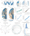
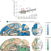
Fig. 2. Prior decoding during the ITI.

a, The Bayes-optimal prior versus the prior decoded from the ORBvl in one session. b, Swanson maps of cross-validated corrected R² for significant areas (Methods) Left, the Ephys map. Right, Ephys and WFI combined. A region is significant if the Fisher combined P < 0.05 on the left map and passes Benjamini–Hochberg correction (1% false-discovery rate) on the right. DN, dentate nucleus; MOp, primary motor area; PAG, periaqueductal gray; PPN, pedunculopontine nucleus; PRNc, pontine reticular nucleus caudal part; PRNr, pontine reticular nucleus. A full list of region names and their abbreviations is available online (https://github.com/int-brain-lab/paper-brain-wide-map/blob/plotting/brainwidemap/meta/region_info.csv). c, Ephys versus WFI results for the dorsal cortex. All areas significantly encode the Bayes-optimal prior in the WFI data (Fisher combined P < 0.05). Blue, significant; orange, not significant; grey, not decoded because we lack quality-controlled data (Methods); white, not decoded due to a lack of recordings or because it was out of the scope of analysis (although both hemispheres were recorded in WFI, only the left is decoded here to match Ephys). d, The corrected R² for Ephys and WFI are significantly correlated (the colour scheme is shown in Extended Data Fig. 5b; shading represents the 95% confidence intervals). e, The proportion of right choices on zero-contrast trials versus cross-validated decoded Bayes-optimal prior from neural activity: higher decoded priors are associated with more right choices (Methods; the shading shows the s.e.m.). f, The corrected R² for decoding the prior from neural activity correlates with the corrected R² for decoding the residual prior (prior minus prior decoded from DLC), indicating that the prior decoded from neural activity is not explained by DLC motor features (the colour scheme is provided in Extended Data Fig. 5a; shading shows the 95% confidence intervals). g, Granger graph at the Cosmos level (Methods and Extended Data Fig. 5) in Ephys showing the bidirectional flow of prior information between the subcortical and cortical regions (right). Left, directed pairs targeting the VISp in WFI data reveal significant feedback from higher-order areas (grey circles) to early sensory regions. h, The proportion of significant directed pairs forming loops of size 3 (orange dashed line) in the WFI (top) and Ephys (bottom) data. The flow of prior information forms more loops than expected by chance (blue null distribution).

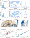
Fig. 3. Encoding of the prior across the brain during the post-stimulus period.

a, Example of neurometric curves for the post-stimulus period from an SCm recording. b, The same as in a, but for the ITI period. c, The correlation between shifts from Ephys and WFI data. Each dot corresponds to one cortical region (two-sided Spearman correlation; the shaded area indicates the 95% confidence interval). d, The post-stimulus shifts are correlated with the ITI R² for both Ephys and WFI data (two-sided Spearman correlation; the colour scheme is shown in Extended Data Fig. 5a; the shading shows the 95% confidence interval). e, Comparison between the corrected post-stimulus neurometric shift in the Ephys and WFI data for the dorsal cortex (left). A region is deemed to be significant if its Fisher combined P value is below 0.05 (Methods). Right, Swanson map of the corrected R² averaged across Ephys and WFI data for areas that have been deemed to be significant given both datasets (using Fisher’s method for combining P values), and after applying the Benjamini–Hochberg correction for multiple comparisons. Blue, significant; orange, not significant; grey, not decoded because we lack quality-controlled data (Methods); white, not decoded because of insufficient recordings or because it was out of the scope of analysis (although both hemispheres were recorded in WFI, only the left is decoded here to match Ephys).

Fig. 4. Action kernel prior.

a, The model frequency and exceedance probabilities for three subjective prior models, using session-wise cross-validation in 107 mice (≥2 sessions; Methods; the error bars show the s.d.). The best model involves filtering recent actions with an exponential kernel. Act. kernel, action kernel; Bayes opt., Bayes optimal; Stim. kernel, stimulus kernel. b, The decay constant for the action kernel across sessions and animals (light purple; median = 5.45 trials, dashed line). The proportion correct for the action kernel as a function of the decay constant is shown (dark purple). The median trial constant aligns with the optimal performance achievable with the action kernel, only 1.9% below the Bayes-optimal performance. c, Performance on zero-contrast trials conditioned on whether the previous action was correct or incorrect, across behavioural models and animal behaviour. Right, the same analysis for a simulated agent using the Bayes-optimal prior decoded from neural data (neural prior) to generate decisions. The performance drop between correct and incorrect previous trials for the neural prior suggests that the action kernel model better accounts for neural activity, consistent with behaviour. Top, WFI data; n = 51 sessions. Bottom, Ephys data; n = 139 mice. Statistical analysis was performed using Wilcoxon signed-rank tests. The error bars show the s.e.m. d, The uncorrected R² is higher when decoding the action kernel prior compared with when decoding the Bayes-optimal prior during the ITI, for the Ephys and WFI modalities. Statistical analysis was performed using Wilcoxon signed-rank tests. e, The weight of the previous actions (purple) and previous stimuli (yellow) on the decoded Bayes-optimal prior, estimated from neural activity (left, Ephys; right, WFI). The dashed lines show the 95th percentile of the null distribution (Methods). f, The correlation between neural inverse decay constants (estimating the temporal dependency of the neural signals on previous actions) and behavioural inverse decay constants (from fitting the action kernel to behaviour). Both Ephys and WFI data show correlations (two-sided Pearson test; Methods; the shading shows the 95% confidence intervals). NS, not significant; *P < 0.05, ***P < 0.001.

Extended Data Fig. 1. Bar plots of the decay constant (τ), amplitude (A) and asymptote (B) of the zero contrast reversal curves across all mice.

The parameters are obtained by fitting the following parametric curve: $p\left(\mathit{correct\; at\; trial\; t}\right)=B$ on the zero contrast pre-reversal trials (the 5 trials before a block switch) and $p\left(\mathit{correct\; at\; trial\; t}\right)=B+(A-B)\cdot e^{-t/\tau }$ on the zero contrast post-reversal trials (the 20 trials after a block switch). τ reflects the reversal timescale. To make up for the limited amount of available zero contrast reversal trials, we fit these curves using a jackknife procedure (see Methods). Bars and error bars indicate jackknife means ± SEM (jackknifing was applied on n = 139 mice). Mice have a significantly longer mean recovery decay constant than the Bayes-optimal observer (4.97 vs 2.43 trials, 2-tailed paired t-test t = 2.94, p = 0.001), while the other parameters are not significantly different. (for A: t = 1.43, p = 0.15 and for B: t = −0.64, p = 0.53) (**p < 0.01, n.s. not significant).

Extended Data Fig. 2. Average wheel speed averaged across sessions before and after stimulus onset.

The decoded time window used for Ephys data is indicated in light grey. For WFI, the data was decoded on the second-to-last frame relative to the stimulus onset, corresponding to a time window that ranges from −198 to −132 ms at the start to −132 to −66 ms at the end, depending on the timing of the last frame before the stimulus onset (this last frame can occur anytime between −132 and −66 ms before the stimulus onset).

Extended Data Fig. 3. Encoding of the prior across the brain during the inter-trial interval.

Sagittal slices corresponding to the main decoding figure presented in Fig. 2b. Left: Ephys only. A region is deemed significant if the Fisher combined p-value is lower than 0.05. Right: Ephys and Widefield combined. Significance for regions is assessed with the Benjamini-Hochberg procedure, correcting for multiple comparisons, with a conservative false discovery rate of 1%.

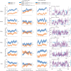
Extended Data Fig. 4. Six examples of neurons significantly encoding the Bayes-optimal prior (***p < 0.001, **p < 0.01, *p < 0.05).

a. Peri-Stimulus Time Histograms (PSTHs) segmented by trials throughout the session. Left column conditions on the Bayes-optimal prior for the right side being less than 0.3 (blue) vs greater than 0.7 (orange). The middle and right columns depict PSTHs for trials under conditions of low certainty (pRight close to 0.5) and high certainty (pRight far from 0.5), respectively. “Med” refers to the median operation. Significance is assessed by testing the difference between the trial wise firing rates (averaging across time bins) of “left” (blue) and “right” (orange) trials with a two-sample Kolmogorov-Smirnov test. b. Spike counts of the neurons (purple line) during the intertrial interval in the [−600, −100] millisecond time window before stimulus onset, along with the Bayes-optimal prior (blue) for a subset of trials within the session (Spearman correlations of the full session are reported on the graphs). All neurons on this panel show a preference for the left side, although, at the population level, we did not observe a bias for either the right or left side. Indeed, we examined the distribution of decoding weights and detected no discernible lateral bias concerning the weight distribution. Testing the significance of the decoder weight in each region yielded adjusted p-values all above 0.2 (Wilcoxon test), after adjusting for multiple comparisons using the Benjamini-Hochberg correction. Additionally, a combined analysis of all weights from the six regions lead to the same conclusion (two tailed signed Wilcoxon test: t = 16732, p-value = 0.31).

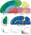
Extended Data Fig. 5

a. Swanson map colour-coded to indicate distinct anatomical regions (Cosmos level). b. Dorsal brain slice recorded with widefield imaging, utilizing the same colour scheme for regional identification. c. Distribution of decoding sessions across different regions as mapped in the Swanson brain atlas. d. Histogram detailing the number of sessions per recording type: Electrophysiology (Ephys) and Widefield Imaging (WFI). The vertical lines indicate median values, with 6 sessions for Ephys and 51 for WFI. e. Dual-axis graph: the coloured lines (left axis) display the p-value of regional significance as a function of the number of decoding sessions, while the black line (right axis) shows the ratio of significant regions relative to the total number of sessions. It is estimated that approximately 10 sessions per region are necessary to identify 95% of significant regions highlighted in the main decoding analysis (refer to Methods section for more details). It is important to recognize that this analysis has limitations: it assumes uniformity across recordings and regions without considering, e.g., variations in effect size or number of units per recording. Despite these limitations, we concentrated on the number of recordings because it is a primary factor that experimenters can directly control.

Extended Data Fig. 6

a. Swanson maps showing corrected decoding R² values for various decoding priors. From left to right: True block prior, log odds ratio of the Bayes-optimal prior, Bayes-optimal prior on a narrower time window (−400 ms to −100 ms), and the Bayes-optimal prior from main Fig. 2b. A region is deemed significant if the Fisher combined p-value is lower than 0.05. b. Correlation analysis comparing Bayes optimal decoding from the extended window (shown in Fig. 2b) with the true block decoding (left panel), the log odds prior (middle panel), and the Bayes-optimal prior from the narrower window (right panel). In the three cases, we have a large correlation between corrected R². c. Comparison of the corrected R² across the four decodings, testing whether the points panel b. are over or below the diagonal (2-tailed signed-rank paired Wilcoxon test, n.s. not significant, ***p < 0.001). d. Bayesian model comparison for 2 behavioural models, the Bayes optimal model, which infers a prior from past observations (see Methods and Supplementary Information), and a model that assumes the true block prior, which is not accessible to the mice. Our analysis shows that the Bayes optimal model more effectively explains the behaviour, with an exceedance probability greater than 0.999.

Extended Data Fig. 7

a. Number of significant sessions for each region represented on the dorsal map for WFI and the Swanson map for Ephys. b. Histograms representing the distribution of the number of significant sessions for each region in both WFI (top) and Ephys (bottom). Note that the number of significant sessions per region in Ephys is low, which prevents us from making robust claims at the regional level. c. Number of units (left) and number of recorded sessions (right) as a function of the decoded R² for the Bayes-optimal prior in Ephys. d. Number of pixels as a function of the decoded R² for the Bayes-optimal prior in WFI. e. Correlations between confounds across modalities. Left panel: Number of pixels in WFI as a function of the number of units in Ephys. Right: Number of pixels as a function of the number of recorded sessions in Ephys. f. Corrected R² for Ephys as a function of the corrected R² for WFI after correcting the WFI R² data for region size. Correcting for the region size in WFI was performed by subtracting the size-predicted R² (from panel d) from the WFI R². Each dot corresponds to one region. All Ephys regions (significant and non-significant) were included in this analysis.

Extended Data Fig. 8

a. Null distribution of the slopes for the proportion of right choice vs decoded prior on zero contrast trials. Slopes were estimated using logistic regression to predict the choice (left or right) as a function of the decoded prior. The null distribution was calculated using 200 pseudosessions. For each pseudosession, pseudoactions were generated from an action kernel behavioural model that was fit to each real session (see Methods for more details). We then obtained pseudoslopes by predicting (with logistic regression) the pseudoactions as a function of the decoded prior. The null distribution was obtained by averaging the pseudoslopes across all sessions (we thus obtain 200 averaged pseudoslopes). The empirical average slope (yellow dashed lines) does not overlap with the null distribution obtained with pseudosessions (blue histogram). Therefore the correlations between the predicted prior and proportion of right choice can not be explained away by spurious temporal correlations or drift in the neural recordings. top: ephys, bottom: WFI. b. Left: Proportion of right choices vs. cross-validated decoded Bayes-optimal prior from neural activity for all contrast strengths in Ephys. Different shades of blue denote different contrast strengths. Main Fig. 2e focused on the zero‐contrast case; here we show the same analysis across all contrasts. Right: Slopes, estimated using logistic regression to predict choice from decoded prior (as in panel a - see Methods). Slopes are strongly modulated by contrast strengths, arguing against a mere perseverative motor bias, which would produce a slope that is invariant across contrasts c. Same as b. but in WFI. d. Proportion of right choices on zero contrast trials as a function of the decoded region-level Bayes-optimal prior. We decoded the Bayes-optimal prior for each region and computed the slope of this decoded prior as a function of the proportion of right choices (corrected using pseudo-sessions). This is the analysis presented in main Fig. 2e but at a region level (significance is assessed when the region-level p-values < 0.05, using Fisher’s method for combining p-values). We observed that the slopes are significant in 17.8% of the regions in Ephys and 90.1% in Widefield, spanning every level of the hierarchy, including LGd, SCm, CP, MOs, and ACAd. It should be noted that the analysis for Ephys includes only 241 regions due to the exclusion of two sessions where the mouse made the same choice on every zero contrast trial. e. Correlation at the regional level between the decoded R² values and the corrected slopes. We find correlations in both modalities. These correlations prompt further investigation into whether they could be explained away by differences in how the Bayes optimal prior versus the action kernel model account for behaviour across sessions. Specifically, sessions that more closely follow the action kernel model could potentially show lower corrected $R^2$ and slopes, as these metrics are calculated using the Bayes optimal prior. In Ephys, we found no correlation between the log Bayes Factor (the difference in the marginal log likelihood between the action kernel and Bayes optimal models at the session level) and the corrected slopes (Spearman correlation: R = 0.05, P = 0.29, N = 412 sessions), with the corrected slopes averaged across regions for each session. In widefield, a small correlation was detected (Spearman correlation: R = −0.34, P = 0.014, N = 51 sessions). However, even after adjusting for the log Bayes factor (by removing the linear prediction of the log Bayes factor from the corrected slope), the correlation between the corrected $R^2$ and the adjusted corrected slope remained strong (Spearman correlation: R = 0.935, P = 4.7 × 10^–15, N = 32 regions). This suggests that the type of behavioural strategy the mice used does not confound the correlation between the corrected $R^2$ and the corrected slope.

Extended Data Fig. 9

a. The decoding R² for the Bayes-optimal prior from neural activity is significantly correlated with the decoding R² for the Bayes-optimal prior from DLC features (Pearson correlation R = 0.18, P = 1.6 × 10^–7). b. Embodiment analysis accounting for both the DLC features and the eye position. Left: Decoding R² for the Bayes-optimal prior from neural activity against decoding R² for the Bayes-optimal prior from DLC features and eye position. The correlation between these two quantities is significant (Pearson correlation R = 0.24, P = 2.5 × 10^–10). Right: DLC + eye position residual decoding R² against neural decoding R². The residual decoding R² values are obtained by first regressing the Bayes-optimal prior from DLC features and eye position, and then regressing the prior residual (Bayes-optimal prior minus Bayes-optimal prior estimated from DLC features and eye position) against neural activity. The neural decoding R² corresponds to the R² when decoding the Bayes-optimal prior from neural activity. The two quantities are strongly correlated (Pearson correlation R = 0.79, P = 5.5 × 10^–141), suggesting that the prior cannot be entirely attributed to a combination of both DLC features and eye position. c. Regressor elimination approach: for each feature, we remove it to measure the decrease in the decoding score compared to the full model (see Methods). The first feature to impact the model significantly when removed is the paw position. In this task, the paws are typically engaged to manipulate the wheel, which in turn adjusts the stimulus. It appears that the paws are positioned differently—likely on the wheel—depending on whether the prior suggests the next side will be left or right. The second key feature was the x-coordinate of the eye position, which aligns with the task setup where the stimulus is positioned along a horizontal plane, indicating that the mice tend to look in the direction suggested by the Bayes-optimal prior. d. Left: decoding R² for the Bayes-optimal prior from neural activity in VISp and LGd against decoding R² for the Bayes-optimal prior from eye position. The correlation between these two quantities is significant (Pearson correlation R = 0.36, P = 0.0163). Right: residual decoding R² against neural decoding R². The residual decoding R² values are obtained by first regressing the Bayes-optimal prior against eye position and then regressing the prior residual (Bayes-optimal prior minus Bayes-optimal prior estimated from eye position) against neural activity in VISp and LGd (see Methods). The neural decoding R² corresponds to the R² when decoding the Bayes-optimal prior from neural activity. The two quantities are strongly correlated (Pearson correlation R = 0.8, P = 7.3 × 10^–11), suggesting that the prior signals in LGd and VISp are not solely due to the position of the eyes across blocks.

Extended Data Fig. 10. Granger causality analysis.

a. Average percentage of significant directed pairs between two regions that reflect the prior across sessions. When considering all pairs of regions encoding the prior significantly, and for which we had simultaneous recordings, we observed that information was significantly exchanged between 71% of these pairs in Widefield imaging and 36% in Ephys. Blue histograms: null distribution. b. Average percentage of significant directed pairs (A- > B) which are reciprocated within the same session by their counterparts (B- > A); we found this to occur 38% of the time in Widefield and 11% in Ephys. Blue histograms: null distribution. (same as in main Fig. 2h). c. Histogram showing the number of sessions for each directed pair and barplot showing the percentage of observed directed pairs (directed pairs with at least one session) versus unobserved pairs. Right: In Ephys, with a total of 242 observed regions, the possible number of pairs amounts to 242 × 241 = 58,322. Of these, approximately 10% of the directed pairs had been recorded simultaneously, but the vast majority (75%) of these pairs appeared in two or fewer sessions, highlighting their scarcity. Left: Widefield provides a richer dataset, because, with 32 regions recorded simultaneously, we can analyse a total of 992 possible directed pairs (32 × 31), most of them available on all sessions. d. Left: Complete connectivity graph from Ephys (p < 0.05 uncorrected for multiple comparisons). When correcting for multiple comparisons, none of the links remains significant. This lack of significant findings post-correction is likely due to the sparse nature of the observations in Ephys (see panel c.). Right: Connectivity graph in Ephys across Cosmos regions (p < 0.05 Bonferroni corrected). p-values across directed pairs of regions are aggregated at the Cosmos level with Fisher’s method (see Methods, identical to main Fig. 2g left). e. Left: Complete connectivity graph from Widefield (p < 0.05 Bonferroni corrected). The graph is densely populated and consequently difficult to interpret. Middle: A partial connectivity graph from Widefield, highlighting significant directed pairs projecting to the Primary Visual Cortex (VISp), as shown in Fig. 2g (right). We uncover feedback connections from higher-order areas such as the Motor Cortex (MOs), Ventral Retrosplenial Cortex (RSPv), Prelimbic Cortex (PL), and Anterior Cingulate Area Dorsal (ACAd) — these regions are marked with grey circles for emphasis — to the early sensory area, the Primary Visual Cortex (VISp). Left: Percentage of sessions exhibiting significant reciprocal connections (A->VISp->A) for sessions in which the Bayes optimal prior could be significantly decoded from both VISp and the previously identified higher-order regions (MOs, RSPv, PL and ACAd). The size of the arrow is proportional to the percentage. Our findings indicate the existence of reciprocal connections in these sessions: 33.3% between MOs and VISp, 16.7% between ACAd and VISp, 20% between PL and VISp, and 18.75% between RSPv and VISp.

Extended Data Fig. 11

a. The average slope of the neurometric curves is significantly different from 0 during the post stimulus period (2-tailed signed-rank Wilcoxon test, t = 9833, P = 1.2 × 10^–5, N = 242 regions) but not during the ITI (t = 13547, P = 0.29, N = 242 regions). Also, neurometric slopes are significantly greater during the post-stimulus period than during the ITI (2-tailed signed-rank paired Wilcoxon test t = 12306, P = 0.028, N = 242 regions) (***p < 0.001, *p < 0.05, n.s. not significant). b. Swanson map of corrected neurometric post-stimulus shifts for Ephys data. c. The corrected post-stimulus shifts and corrected ITI shifts are significantly correlated in both Ephys (Spearman correlation R = 0.19, P = 0.0026, N = 242 regions) and WFI (Spearman correlation R = 0.57, P = 0.0007, N = 32 regions).

Extended Data Fig. 12

a. The neural decoding R² for the stimulus side and the Bayes-optimal prior are significantly correlated across brain regions (Spearman correlation R = 0.29, P = 2.4 × 10^–5). b. Swanson maps and dorsal cortical views of brain regions encoding the Bayes-optimal prior (blue, upper) and the stimulus side (green, lower) significantly based on Ephys data.

Extended Data Fig. 13

a. Bayesian model comparison for 11 behavioural models, considering the possibility of one step repetition bias (i.e. a tendency to repeat the previous choice), multi-step repetition bias (i.e. a tendency to follow an exponentially decaying average of past choices), and, for the stimulus kernel model, the presence of positivity and confirmation biases as asymmetric learning rates (accounting for the possibility to learn differently from positive versus negative rewards and from information that confirms versus contradicts existing beliefs. See Methods for more details on the Bayes-optimal, action kernel and stimulus kernel models and Supplementary information for the formal equations of the repetition bias and asymmetrical learning rates. Model frequency (the posterior probability of the model given the subjects’ data, left panel) and exceedance probability (the probability that a model is more likely than any other models, right panel) are shown. The action kernel model offered the best account of the data even when including models with repetition, positivity and confirmation biases (p_exceedance > 0.999). b. Bayesian model comparison for two behavioural models, the action kernel and a variant that operates only during 0% contrast trials (by calculating an exponentially decaying average of chosen actions at 0% contrast trials). Our comparisons indicate that the action kernel, updating across all contrasts, more effectively explains behaviour (exceedance probability > 0.999), suggesting that mice do not limit their subjective prior estimations to 0% contrast trials alone. c. Performance on zero contrast trials, distinguishing whether the preceding action was correct or incorrect and considering that the previous contrast was non zero. This analysis mirrors the main analysis in Fig. 4c but is specifically restricted to previous trials with non-zero contrast. When considering behaviour within blocks, an agent using an action kernel prior should show a higher percentage of correct responses following a correct, block-consistent action compared to an incorrect one. This is because, on incorrect trials, the prior is updated with an action corresponding to the incorrect stimulus side. Even when limited to previous trials with non-zero contrast, there is a notable difference in the probability of making a correct decision following an incorrect vs. a correct choice (Wilcoxon paired test, t = 11734, P = 1.1 × 10^–15). This finding is confirmation that mice update their priors using information from all contrast levels, not solely zero contrast trials. d. Psychometric shift during both the first 90 trials (unbiased) and the other trials (biased) for animals and the action kernel. This shift is determined by analysing two psychometric curves, one conditioned on the action kernel prior being above 0.5 (favoring the right side) and the other conditioned on the action kernel prior being less than 0.5 (favoring the left side). We fit psychometric functions to these curves, and then calculate the psychometric shift as the vertical displacement of these curves at zero contrast. As predicted by the action kernel model, the analysis reveals a significant positive psychometric shift during the unbiased phase (first 90 trials). Furthermore, the shift in the behavioural data is less pronounced during the unbiased period compared to the biased period because the stimuli are more balanced in the unbiased phase, keeping the subjective prior closer to 0.5. Specifically, when distinguishing the trials that favour the right side (action kernel prior above 0.5) from those favoring the left side (action kernel prior below 0.5), the underlying action kernel priors remained close to 0.5 during the unbiased period. However, the presence of significant and comparable shifts between the animals and the action kernel model during the unbiased period indicates that mice exhibit a behavioural shift during the unbiased trials.

Extended Data Fig. 14. Same analysis as in Fig. 4c,e, but for three specific brain regions using Ephys (SCm, CP, VPM) or WFI data (right column, MOp, VISp, MOs) (*p < 0.05, **p < 0.01, ***p < 0.001).

For the influence of past actions on the decoded Bayes-optimal prior, significance is assessed in the same way as in the main Fig. 4e (see Methods). For the asymmetry effect, the effect being observed on a brain-wide level, we performed a 1-tailed signed-rank Wilcoxon paired test for assessing significance on the region level.

Extended Data Fig. 15

a. Behavioural inverse decay constants, obtained by fitting the stimulus kernel model to the behaviour, as a function of the neural inverse decay constants, obtained by estimating the temporal dependency of the neural signals with respect to previous stimuli (see Methods). The neural and behavioural inverse decay constants are not significantly correlated for either Ephys (Pearson correlation R = 0.03, P = 0.71) or WFI (Pearson correlation R = −0.04, p = 0.82). b. Hierarchical modelling of the neural and behavioural inverse decay constants (also referred to here as learning rates). The parameter ${\mu }_j$, defined for each mouse j, is the slope (the multiplicative coefficient) of the linear regression predicting the neural learning rate from the behavioural learning rate (on the sessions of mouse j). These parameters ${\mu }_j$ are sampled from a common population level prior with mean ${\mu }_0$.The parameter ${\mu }_0$, defined at the population level, characterizes an overall relationship between neural and behavioural learning rates. We found that the relationship between neural and behavioural learning rates is significantly positive for the action kernel model (top row), both in electrophysiology (left column) and in widefield imaging (right column), which is not the case for the stimulus Kernel model (bottom row). Furthermore, when testing the difference in means of the population level parameter ${\mu }_0$ between action and stimulus kernels, we found that it was significantly greater for the action kernel, both in Ephys and in WFI. Significance was assessed by estimating the means of the ${\mu }_0$ distributions for the action and stimulus kernels with the BEST Bayesian test. In both Ephys and WFI, we found that $p(\overline{{\mu }_0^{\mathit{actKernel}}}>\overline{{\mu }_0^{\mathit{stimKernel}}})=1$ with $\overline{{\mu }_0^{\mathit{actKernel}}}$ and $\overline{{\mu }_0^{\mathit{stimKernel}}}$ the means of the ${\mu }_0$ distributions for the action and stimulus kernels, respectively. Regarding the effect sizes, with the same BEST procedure, we find an effect size of 2.53 in Ephys and 1.96 in widefield (effect sizes greater than 1.3 are commonly considered to be very large). See Supplementary Information for the full specification of the hierarchical generative model. c. Correlation, at a region level, between neural inverse decay constants (estimating temporal dependency of the neural signals on previous actions), and behavioural inverse decay constants (from fitting the action kernel to behaviour). A decay constant is estimated for each pixel (as in Fig. 4f, refer to Methods), but now, averages are taken across pixels for each session and specific region. In the analysis Fig. 4f, session-level learning rates were obtained by averaging across all pixels, regardless of region identity. Left: Regions with a significant correlation between behavioural and neural inverse decay constants. As expected, only positive correlations emerge as significant. Right: Correlation between behavioural and neural inverse decay constants is correlated with the prior decoding corrected R² from the same regions. These two quantities were found to be also correlated (R = 0.46, P = 0.008). In other words, regions in which the prior decoding R² is large are also regions which best reflect the behavioural decay constant, i.e., these are the regions that are best correlated with the animals’ cognitive strategies as assessed by the lengths of the action kernels. We did not repeat this analysis with the electrophysiology recordings because we only have a very limited number of significant sessions per region (1-2 for most regions, as opposed to around 20 sessions per region for the WFI data - see Extended Data Fig. 7a,b).

References

1. Knill, D. C. & Pouget, A. The Bayesian brain: the role of uncertainty in neural coding and computation. Trends Neurosci.27, 712–719 (2004). - PubMed
1. Ernst, M. O. & Banks, M. S. Humans integrate visual and haptic information in a statistically optimal fashion. Nature415, 429–433 (2002). - PubMed
1. Jacobs, R. A. Optimal integration of texture and motion cues to depth. Vision Res.39, 3621–3629 (1999). - PubMed
1. Mamassian, P., Knill, D. C. & Kersten, D. The perception of cast shadows. Trends Cogn. Sci.2, 288–295 (1998). - PubMed
1. Weiss, Y., Simoncelli, E. P. & Adelson, E. H. Motion illusions as optimal percepts. Nat. Neurosci.5, 598–604 (2002). - PubMed