Anatomical circuits for flexible spatial mapping by single neurons in posterior parietal cortex

Abstract

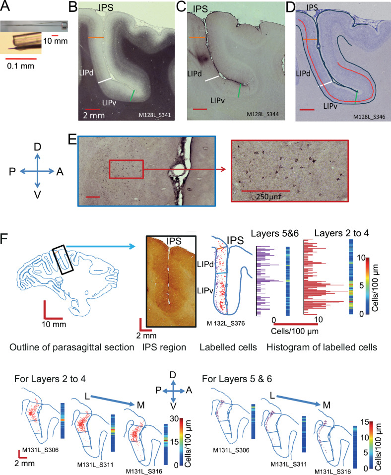
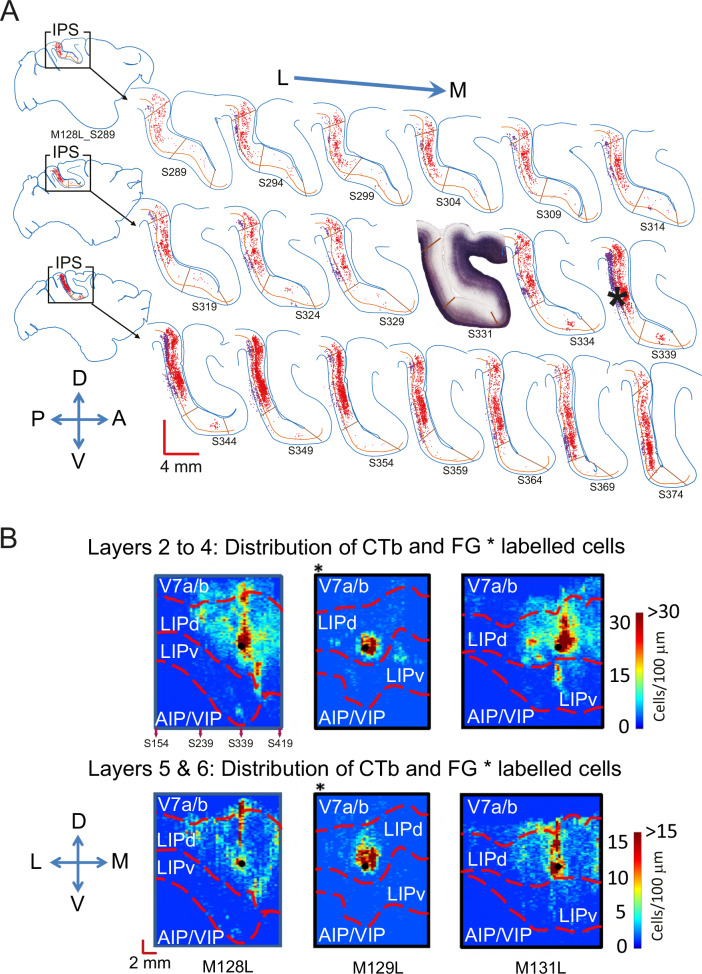
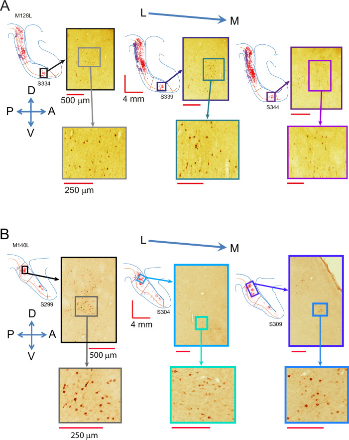
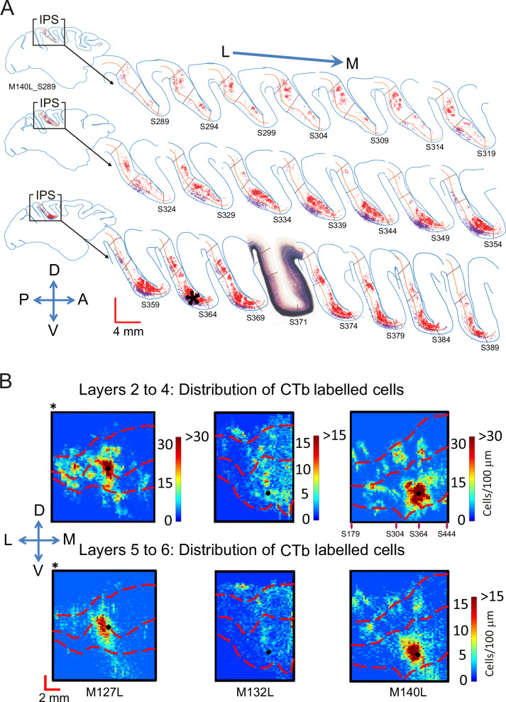
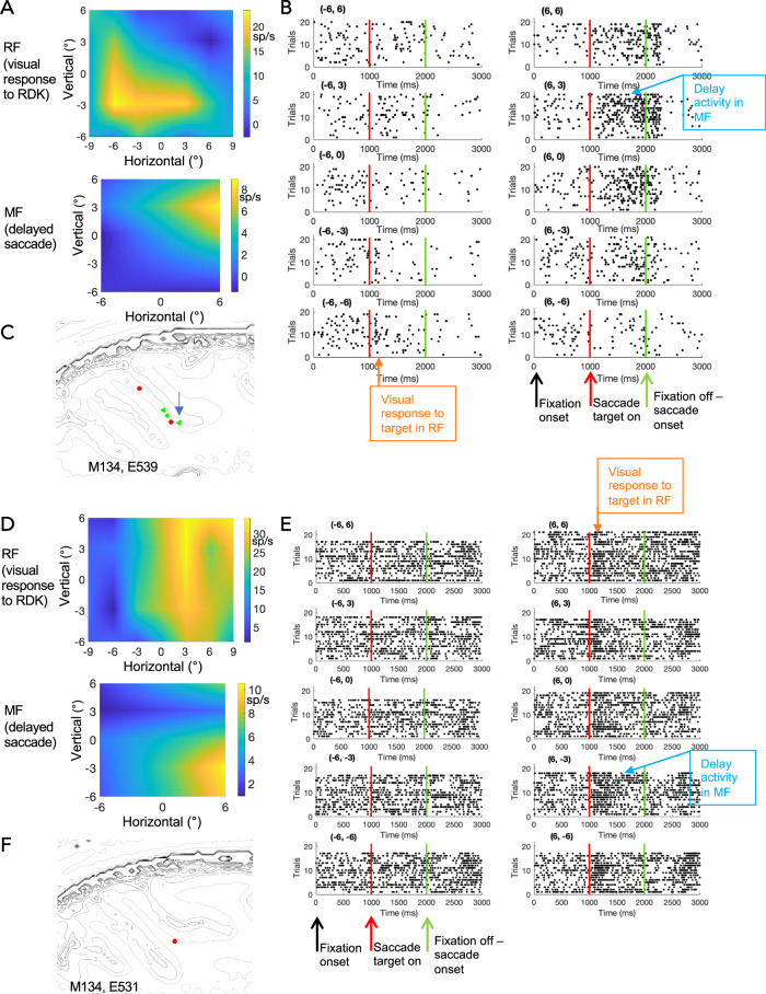
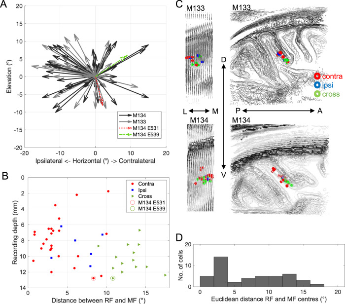
Primate lateral intraparietal area (LIP) has been directly linked to perceptual categorization and decision-making. However, the intrinsic LIP circuitry that gives rise to the flexible generation of motor responses to sensory instruction remains unclear. Using retrograde tracers, we delineate two distinct operational compartments based on different intrinsic connectivity patterns of dorsal and ventral LIP. These connections form an anatomical loop with a sensory-like, point-to-point projection from ventral to dorsal LIP and an asymmetric, widespread projection in reverse. In neurophysiological recordings, LIP neurons exhibit motor response fields spatially distinct from their sensory receptive field. Different associations of motor response and receptive fields in single neurons tile visual space. Ventral LIP neurons tend to have motor response fields distant from their sensory receptive fields. This circuit provides the neural substrate to generate the dynamic processes for flexible allocation of attention and motor responses in response to salient or instructive visual input across the visual field.

Fig. 1. Tracer injections and analysis.

A Injections were placed via a glass capillary tube filled with tracer which was glued to a tungsten electrode for recording neural activity (reproduced with permission). B, D Parasagittal sections through the intraparietal sulcus. B This section was stained for myelin using the Gallyas method. LIPv is identified histologically by the more dense, extended intracortical myelin, LIPd by the two bands. C Nearest parasagittal section (to B) showing the CTb injection site in LIPd, taking a posterior approach. For LIPv, we took either a posterior approach (two animals) or a dorsal approach (one animal). D Nearest Nissl-stained section (to C) identifying the border (red line) between layers IV and V to be able to distinguish potential differences in the pattern of connectivity in supra- and infragranular layers. E Section stained for CTb shows the retrogradely labelled neurons. The high-resolution image (right) reveals the shape and granulated fill of individual neurons, which were the criteria for accepting a neuron as labelled. F Method for the data transformation of CTb labelled cells from an individual parasagittal sections into 3D maps of intrinsic LIP connectivity using two example injections. Top: Labelled cells were converted to density measures in 100 µm bins along the dorso-ventral axis, separately for supragranular (layers 2–4) and infragranular layers (5 and 6) (example M132L after LIPv injection). No smoothing across bins took place. Bottom: Then, data were aligned section-by-section along the medio-lateral extent of LIP (example M131L after LIPd injection). A – anterior, P – posterior, L – lateral, M – medial, D – dorsal, V – ventral.

Fig. 2. Neurons in LIPd receive topographic input from a single site in LIPv but widespread input from within LIPd.

A A one-in-five series of parasagittal sections shows the distribution of labelled cells after a CTb injection into LIPd in the left hemisphere of one animal (M128L). Retrogradely labelled neurons can be found throughout the layers and the extent of LIPd, but there is only one clear cluster of labelled cells in LIPv that project to the injection site. The densest label in LIPd is medial to the injection site. The inset section shows the myelin definitions of LIPv and LIPd from an alternate series. Red cells are in supragranular layers I-IV, purple cells in infragranular layers V-VI; * denotes the injection site. See Fig. 3A as well as Supplementary Figs. 2 and 3 for histological images before annotation and further Gallyas sections. B The plots summarise the 3D-pattern of label (dorso-ventral; medio-lateral; supragranular and infragranular layers) across all three animals with a tracer injection into LIPd (denoted as filled black dot). M129 (*) received an injection of the retrograde tracer Fluorogold, M128 and M131 of CTb. All three animals show an LIPd-intrinsic, wide-spread network of neurons that project to the injection site in area LIPd itself. They also all show a single cluster of labelled cells in LIPv indicative of a topographic input from LIPv to LIPd. For M128L, we show section numbers in the density map relating to the sections in A. L – lateral, M – medial, D – dorsal, V – ventral, A – anterior, P – posterior.

Fig. 3. Histological images of clusters of labelled cells.

A Histological sections showing the retrogradely labelled cells of the cluster in LIPv for the brain presented in Fig. 2A after an injection in LIPd, at low and high magnification. B Histological sections showing the retrogradely labelled cells of a cluster in LIPd for the brain presented in Fig. 4A after an injection of retrograde tracer in LIPv.

Fig. 4. Neurons in LIPv receive wide-spread input from within LIPv and from several cell clusters in LIPd.

A A one-in-five series of parasagittal sections shows the distribution of labelled cells following a CTb injection in LIPv (M140L). Retrogradely labelled neurons can be found in supra- and infragranular layers across LIPv. In LIPd, several clusters of labelled cells are seen throughout the medio-lateral extent of LIPd. The inset section shows the myelin definitions of LIPv and LIPd from an alternate series. Red cells are in supragranular layers 2–4, purple cells in infragranular layers 5 + 6 with largely similar results; * denotes the injection site. B Plots summarise the 3D-pattern of label across all three animals with a tracer injection into LIPv (at the LIPd/v border for M127L *). All three animals show an LIPv-intrinsic wide-spread network of neurons that project to the injection site as well as multiple clusters of labelled cells in LIPd projecting to LIPv. For M140L, we show section numbers underneath the density map related to the sections depicted in A. See Supplementary Fig. 4 for a histological image of M132L before annotation. L – lateral, M – medial, D – dorsal, V – ventral, A – anterior, P – posterior.

Fig. 5. The RF and MF of example LIP neurons.

A–C Data from one LIP neuron. A This example cell has a visual receptive field (RF) as mapped with a RDK stimulus (top) that is spatially distinct from its  motor response field (MF) (bottom) in a delayed saccade task. Scale is relative to central fixation at 0°,0°. See Supplementary Fig. 5 for unsmoothed representations of the RF and MF maps. B The raster plots for the delayed saccade task for the MF shown in (A). Each plot represents a saccade target position. Degrees of visual angle from central fixation are given above the plot. Each line represents a trial with dots as individual spikes. The neuron shows a brief response to the onset of the saccade targets (a dot) at positions -6°,-3° and -6°,-6°, in the region where the sensory RF was localised to in the separate mapping experiments with an RDK (see A). But the delay activity was recorded while the animal was waiting to carry out a saccade to targets at +6, +3 and +6, 0. C Grey outlines highlight tissue boundaries derived from the structural MRI obtained from the individual animal. The coloured dot gives the projected location of the recorded example cell depicted in (A, B); the colour identifies the type of MF-RF relationship (green: MF and RF located in different visual hemifields). Where we recorded multiple cells in the same parasagittal plane, an arrow points to the example neuron. D–F Data from another LIP neuron. Same conventions as in (A–C). F The coloured dots give the projected location of the recorded cells, the colour identifies the type of MF-RF relationship (red – both contralateral, green – across different hemifields). More examples can be found in Supplementary Fig. 6.

Fig. 6. Distribution of MFs and RFs of LIP neurons.

A For this figure, we projected all RF centres of LIP neurons to the centre of the graph (0°, 0°) and plotted the direction and relative distance of the MF centres as an arrow. This figure includes all LIP cells that we could map qualitatively online (n = 111). Some RF and MF centres are very close to each other, others quite far removed. As most RFs are found in the contralateral visual hemifield and about half of the MFs on the ipsilateral side, many arrows point to the left. Overall, a large range of different associations can be found, which tile the mapped visual field. Colour-coded are the examples from Fig. 5. B Recording depth (out of guide tube, 2 mm into the brain) was plotted against distance between RF and MF centres for LIP neurons with a significant RF and MF (n = 45). The colour and shape identify the type of MF-RF relationship (red circle: MF and RF in the contralateral visual hemifield; blue square: MF and RF ipsilateral; green triangle: MF and RF in different visual hemifields). C Spatial location of all LIP neurons with significant RF and MF for the two monkeys (M133, M134). LIP neurons with RF and MF across the two hemifields tend to be located more ventrally. Grey outlines depict tissue boundaries (extracted with Matlab using contourslice) for stacked parasagittal sections in a structural MRI volume centred on LIP. Views are either from posterior (left) or from the side (right). D Distribution of absolute distances between RF and MF centres for LIP neurons with a significant RF and MF (n = 45). In our sample, many LIP neurons have overlapping RFs and MFs but a considerable fraction can be as far apart as 12–18 degrees.

Fig. 7. Summary of LIP intrinsic connectivity, the wider cortical network and the proposed circuit for processing perceptual decisions about 3D motion in macaques.

A This diagram summarises the key findings of the intrinsic connectivity pattern between LIPd and LIPv from this study. LIPv, previously shown to be topographically organised, sends a point-to-point projection to LIPd (blue arrows). In turn, each point in LIPv receives inputs from a number of different regions within LIPd (white arrows). Within both compartments, there is widespread connectivity. B Illustration of selected, previously established cortico-cortical in- and outputs to LIPv and LIPd. Extrastriate visual area V5/MT projects exclusively to LIPv, not LIPd, while ventral stream visual area V4 has a stronger projection to LIPd^,. The frontal eye fields (FEF) send a feedforward-type projection to LIPd, and a feedback-type projection to LIPv. These connections with FEF are reciprocal. C Illustration of the proposed processing scheme for perceptual decisions about 3D structure-from-motion stimuli, based on input of perceptual evidence represented in area V5/MT^, projected in a topographic fashion to LIPv. This input can convey perceptual signals about direction of motion and 3D depth localised to specific locations in the visual field. The intrinsic network between LIPv and LIPd can map one input (topographically mapped in LIPv) to other potential visual field locations through the connectivity loop with LIPd. The specific association between the sensory RF and saccade MF might be achieved gradually in a recurrent network. Interconnected with a feedforward connection into LIPd and receiving input from LIPv, FEF signals could support an attentional shift from stimulus to choice target representations and thus facilitate the association of the stimulus with a specific choice target. The map of planned saccade target locations in FEF is thus connected to the visual perceptual map in V5/MT through the circuitry in LIP. The specific associations of RF and MF in single neurons we found could be the product of the daily visual experience of the animals directing saccades to salient visual features and the specific training the animals underwent to learn to make perceptual decisions about 3D structure-from-motion objects. Arrows intrinsic connectivity: blue – projection to LIPd injection site, white – to LIPv injection site; arrows inter-area connectivity: black – feedforward, grey – feedback.

Fig. 8. Positioning and alignment of neurophysiological penetrations.

A shows a view into the vertical chamber (blue circle) implanted on the skull of one animal (M134). It is viewed with a superimposed, schematic grid as used for stereotactic penetrations in the neurophysiological experiments. The filled grey circles indicate the locations of the example penetrations/cells in the following panels. B shows a sagittal slice from the pre-surgical MRI. C Neurophysiological white matter and grey matter maps along a posterior-to-anterior row of penetrations in one parasagittal plane (x = 3 in the chamber grid) and depth from entry into the cortex. Red-filled circles and green-filled triangles indicate the recorded cells (convention as in Figs. 5 and 6: red – RF and MF both contralateral; green – RF and MF in different visual hemifields). On each penetration, we identified borders of grey matter and white matter by background neuronal sound and spiking activity. We plotted a black line indicating clear grey matter and a blank indicating the white matter (no response of cells and background sound). The dashed horizontal lines represent entry to cortex and putative LIPd/LIPv border respectively. D The black-blank lines from (C) were aligned with the borders between grey matter and white matter in the pre-surgical MRI shown in (B).

References

1. Ibos, G. & Freedman, D. J. Sequential sensory and decision processing in posterior parietal cortex. Elife6, e23743 (2017). - PMC - PubMed
1. Andersen, R. A. & Cui, H. Intention, action planning, and decision making in parietal-frontal circuits. Neuron63, 568–583 (2009). - PubMed
1. Colby, C. L. & Goldberg, M. E. Space and attention in parietal cortex. Annu. Rev. Neurosci.22, 319–349 (1999). - PubMed
1. Glimcher, P. W. Decisions, Uncertainty and the Brain. The Science of Neuroeconomics (MIT Press, 2003).
1. Gold, J. I. & Shadlen, M. N. The neural basis of decision making. Annu. Rev. Neurosci.30, 535–574 (2007). - PubMed
LinkOut - more resources