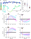
[Preprint]. 2025 Sep 1:2025.08.27.672631.
doi: 10.1101/2025.08.27.672631.

Mice navigate scent trails using predictive policies

Affiliations

Mice navigate scent trails using predictive policies

Siddharth Jayakumar et al. bioRxiv. .

Abstract

Animals actively sense their environment to extract features of interest to guide behaviors. For mammals, odors are prominent environmental features which are sampled by active modulation of sniffing and orofacial orientation. We sought to understand the strategies that mice use to navigate surface-bound odor cues. We presented mice with dynamic, non-repeating odor trails using a paper treadmill, and observed their behaviors as they collected rewards offered randomly along the trail. By combining high-speed videography over long distances with quantitative behavioral analyses, we find that mice rapidly learn to track odor trails persistently and precisely. Mice with a single nostril blocked can track odor trails, but with a lateral bias and lower precision than control animals. Tracking is severely impaired in animals with both nostrils intact but with interhemispheric communication disrupted by anterior commissure transection. Respiration measurements revealed that a sniff close to the trail triggers a rapid turn towards the trail, a reaction that is lost in commissure-cut animals. Importantly, trail tracking is not simply reactive but involves adaptation to and retention of a short-term memory of the trail geometry and statistics. Our results, recapitulated by a Bayesian inference model, indicate that mice combine immediate sensory information with an internal model of the odor environment to follow odor trails efficiently.


Figures
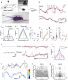
Figure 1:
Figure 1:. Mice rapidly learn to follow continuous trails.
(a) Schematic of the custom-built paper-based treadmill. M1 & M2: rollers, with M1 coupled to a DC motor; C1 & C2: cameras; P: printhead that houses the printhead. The mice are restricted to the width of the chamber with walls made of acrylic that allow imaging with cameras. Odors are delivered using a printhead or a brush, controlled by stepper motors, allowing us to deliver varying geometries on the fly. Key points on the mouse (snout, right and left ear bases as well as base of the tail) identified using DeepLabCut (Mathis et al., 2018) are shown in magenta. b) Examples showing the trajectory of a mouse on day 1 (naïve) and on day 6 (expert) following a trail. The trail is shown in black. The snout is shown in purple, with a rhombus joining the snout, ears and base of the tail in pink. c) Distributions showing the snout deviation from 6 mice when naïve (day 1) vs when they have become experts (day 6), ***p<0.001, Kolmogorov–Smirnov test. Each line indicates a unique animal. d) The same data shown in panel c, but subsampled to include only points closer than 2.5cm on either side of the trail, numbers indicate percentage tracking. (e-h) Performance metrics of following a trail in naïve and expert mice. Each dot represents an individual animal, except in g where each colored dot represents an animal. (e) Root mean square deviations from the trail either in naïve or expert animals. ***p<0.001, Two-tailed Wilcoxon rank-sum test. (f) Mean number of epochs, ***p<0.001, Two-tailed Wilcoxon rank-sum test. (g) Length of each epoch, ***p<0.001, Mann-Whitney U test and (h) Elevation of the snout from the paper floor, *p<0.05, Two-tailed Wilcoxon rank-sum test. (i) Left: 2 example trails presented to mice. Right: Examples of a mouse following either a simple straight or a tortuous trail. (j) Distributions of snout deviations for 5 mice when following either a simple or a tortuous trail. (k) Examples of trail tracking in naïve or expert mice, with the vertical elevation of the snout mapped on to the tracks (colormap representing snout elevation shown to the right). (l, m) Distributions showing snout occupancy in 3d space in naïve mice (l) and when they have become experts (m).
Figure 2:
Figure 2:. Coordination of bilateral inputs is helpful for accurately following trails.
(a) Example time series from a thermocouple in a sham operated and a nostril stitched mouse. The thermocouple signal was at zero when the corresponding nostril was blocked. The arrow indicates inhalation. This was used to confirm that the nostril occlusion prevented airflow in that side. (b) Example trajectory from a mouse following a trail either after a sham stitch or when the left nostril was stitched. (c) Distributions of the deviations of the snout from the trail from either mice where there was a sham stitch or when the nostril was stitched, **p<0.01, Kolmogorov–Smirnov test, numbers indicate percentage tracking. (d) Histological evidence for the transection of the anterior commissure. (e-g) Example trajectory from a mouse with either sham surgery, one with the anterior commissure transected and with an animal where the nostril was stitched post severing the anterior commissure. Inset shows zoomed in sections. (h,i) Distributions of snout deviations from at least 5 mice in conditions shown in (e,f,g) for all periods of behavior (h) or selected periods when mice were within 3cm of the trail (i),***p<0.001, Kolmogorov–Smirnov test. Numbers indicate percentage tracking.
Figure 3:
Figure 3:. Modulation of respiration during trail tracking allows quick turns at trail edges.
(a) Example trajectory of a mouse either following a trail or when there is no trail. Inhalations are shown in color. The colormap shows instantaneous respiration rate. (b) Average respiration rates in different conditions, **p<0.01, Kruskal-Wallis ANOVA with post hoc Mann-Whitney U tests using Bonferroni multiple comparisons correction. (c-f) Average mouse trajectories showing snout (large circles), shoulder and base of the tail, joined by lines. The red dot indicates the anchor point for the averages, when the mouse snout was within 1 – 2cm of the trail after crossing it. Pink traces are averages when an inhalation was detected at t = 0, and cyan are when there is no inhalation at t = 0. Left and right panels are separate averages for trail crossings in opposite directions. Trail of 0.5cm is shown as a gray line. (c, d) is from wild type mice (at least 27 stretches from 12 mice) and (e, f) shows data from mice where the anterior commissure was transected (at least 28 stretches from 8 mice).
Figure 4:
Figure 4:. Mice use memory of previously encountered trail statistics.
(a) Example trajectories from mice encountering a break while tracking a trail that is either straight (top) or tortuous (bottom). (b) Casting amplitude from 7 stretches from 5 mice encountering a break when following a straight trail. (c) Casting amplitude from 7 stretches from 5 mice encountering a break either when following a straight trail (black) or a more tortuous trail (red). (d) Snout deviations over time as mice encounter a sudden turn while following a trail. (e) Averages of the integrated maximum snout deviations over 2 seconds after encountering a turn after different periods of following a straight trail. (*p<0.05, Kruskal-Wallis ANOVA with post hoc Mann-Whitney U tests using Bonferroni multiple comparisons correction). Each point is for one session from one mouse. (f) Example trajectories from straight sections of a trail before or after encountering noise patterns in the trail (g) Maximum snout deviation in sections where the trail was straight preceded by trails of varying noise patterns. (h) Maximum snout deviation in a straight section of the trail immediately after encountering a trail with a root mean squared deviation of 4.1cm. The average maximum snout deviation from 9 expert mice that have not faced noisy trails are shown in green. The R2 value indicates goodness of fit, p-value=0.9032 (Chi-squared test). The best fitting time constant was 18.4 seconds.
Figure 5:
Figure 5:. An agent using memory reproduces many facets of tracking behavior.
(a-d) Example trajectories of an agent using a Gaussian Process Regression to estimate the trail from previous contacts with the trail. The virtual trail is shown in black, the agent’s trajectory in orange, the agent’s trail encounters as sky blue dots, the agent’s heading estimate in a sky blue line and the posterior uncertainty of the trail position (± 2σ, where σ is the standard deviation output by the GPR at each point) in gray cones. The example trajectories are from the agent following a) a simple straight line, b) a simple trail with breaks, c) curves of low tortuosity and d) curves of high tortuosity. (e) Deviations from the trail as shown by means ± s.e.m. are from 30 simulations, show that the agent is accurate in following trails. (f and g) Example trajectories of the agent encountering a break while following trails of two types of curvature. (h) Casting amplitudes measured from 30 simulations as shown by means ± s.e.m. show that the agent casts more widely when encountering a break following the trail of higher curvature. ***p<0.001, Mann-Whitney U test. (i and j) Example trajectories from an agent following a straight section of a trail after encountering either low tortuosity (i) or high tortuosity (j). (k) Snout deviations over time from agents following a trail. The deviations are rom straight sections of the trail. The deviations are significantly higher when the trail was preceded by the curves of higher tortuosity. ***p<0.001, Mann-Whitney U test.

References

    1. Aitchison L, Lengyel M. 2017. With or without you: predictive coding and Bayesian inference in the brain. Curr Opin Neurobiol 46:219–227. doi: 10.1016/j.conb.2017.08.010 - DOI - PMC - PubMed
    1. Álvarez-Salvado E, Licata AM, Connor EG, McHugh MK, King BM, Stavropoulos N, Victor JD, Crimaldi JP, Nagel KI. 2018. Elementary sensory-motor transformations underlying olfactory navigation in walking fruit-flies. eLife 7:e37815. doi: 10.7554/eLife.37815 - DOI - PMC - PubMed
    1. Arulampalam MS, Maskell S, Gordon N, Clapp T. 2002. A Tutorial on Particle Filters for Online Nonlinear/Non-Gaussian Bayesian Tracking. IEEE TRANSACTIONS ON SIGNAL PROCESSING 50.
    1. Attneave F. 1954. Some informational aspects of visual perception. Psychological Review 61:183–193. doi: 10.1037/h0054663 - DOI - PubMed
    1. Barlow HB. 1961. Possible principles underlying the transformations of sensory messages In: Rosenblith WA, editor. Sensory Communication. Cambridge, MA: MIT Press. pp. 217–234.

Publication types

LinkOut - more resources