Population-genomics reveals a dual ancestry of grizzly bears

Abstract

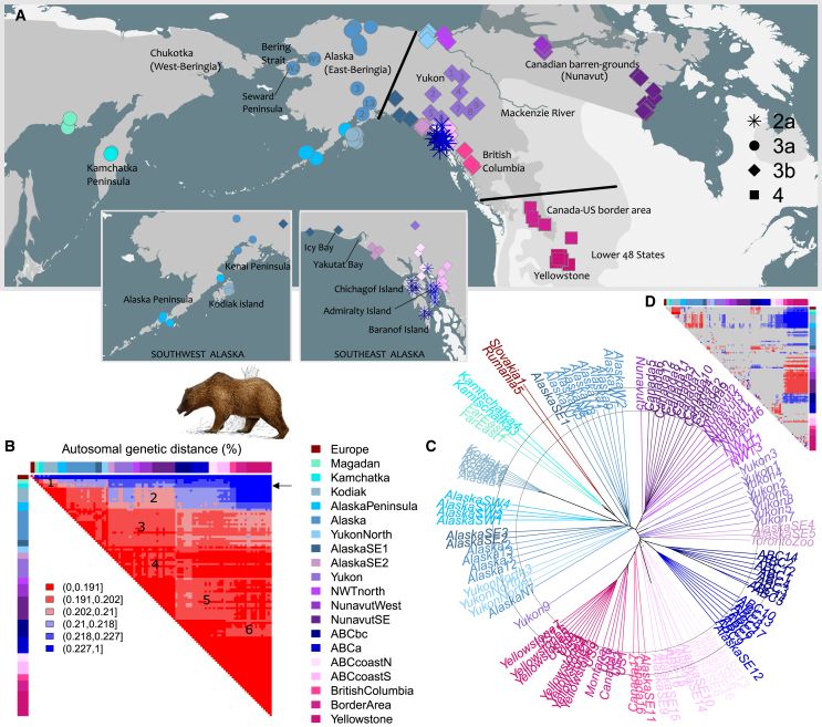
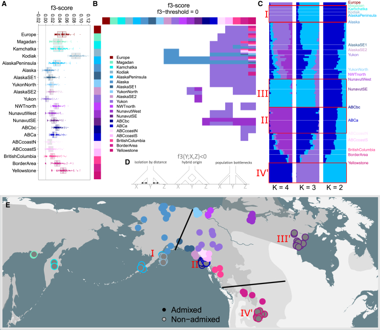
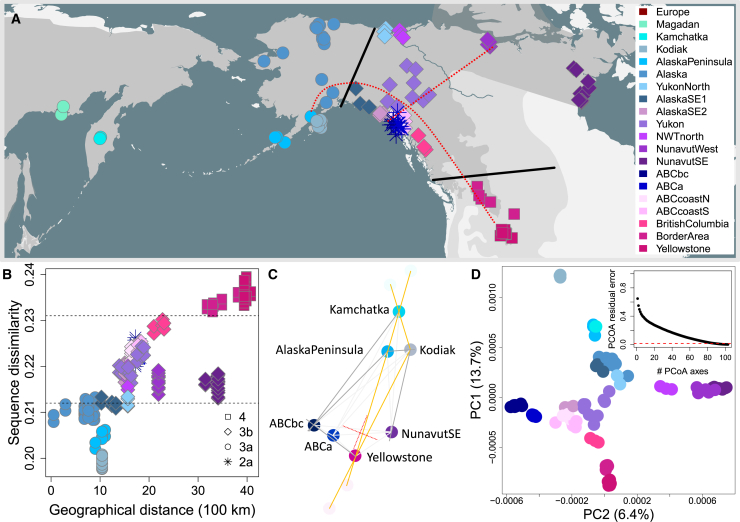
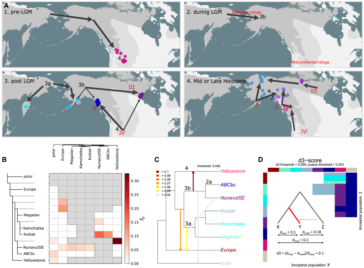
Genetic variation among populations reflects both past demographic events and current population connectivity. We investigate the primary drivers of genetic differentiation in American brown bears (Ursus arctos) using 108 nuclear genomes. Our analyses reveal that genome-wide distances conform to neither an isolation-by-distance model nor a bifurcating tree structure. Building on previous ancient-DNA and fossil studies, we propose a demographic scenario in which continent-wide admixture during the Late Holocene has obscured, but did not erase, the genetic legacy of earlier colonization waves and subsequent gene flow events. The most persistent signals of these past events are striking genetic similarities between populations now separated by water barriers, including Kamchatka and Southwest Alaska bears. Our findings underscore that convergence to migration-drift equilibrium takes time, making genetic distance an imperfect proxy for present-day population connectivity.

Keywords: Animals; Biological classification; Evolutionary history; Phylogenetics.

Graphical abstract

Figure 1

North American brown bear population structure does not fit a bifurcating model (A) Sample distribution. Dark and light gray: present-day and historic geographical range of brown bears (https://www.iucn.redlist.org). Symbol types indicate mtDNA haplotypes. Black lines indicate mtDNA discontinuities. (B) Distance matrix. Annotated heatmap depicting autosomal sequence dissimilarity, E(p), between pairs of individuals. The transition from blue to red colors highlight that Kodiak bears and Alaska Peninsula bears (combinedly “Southwest Alaska”) cluster separately from other North American brown bears, with remaining Alaskan bears clustering intermediate. The arrow denotes the cross-section shown in Figure 3B. Numbers indicate major violations from a bifurcating tree model, and indicate excess allele sharing between populations of (1) Southwest Alaska and Far East Russia, (2) Southwest Alaska and Nunavut, (3) central Alaska and Nunavut as well as Yukon and Southeast Alaska, and a shortage of allele sharing between populations in (4) Yukon and Nunavut, (5) Southeast Alaska and Nunavut, and (6) lower 48 states and Baranof/Chichagof Islands. (C) Autosomal dendrogram. Unrooted multi-locus bioNJ dendrogram (“tree of individuals”), constructed from the distance matrix in (B). The concentric circles have been added to aid visual interpretation, and highlight the distinctness of Southwest Alaskan bears, and to a lesser extent of central Alaska bears. Note also the slightly elongated branches leading to bears of Baranof and Chichagof Islands (“ABCbc”), which indicate slightly elevated genetic distances to other brown bears, resulting from gene flow from polar bears and their isolation from the mainland. The long internal branch of Kodiak bears signals a population bottleneck, which resulted in a loss of genetic variation. (D) Residual error matrix, depicting the difference between tip-to-tip path lengths of the dendrogram and the corresponding entries in the distance matrix. Note, for instance, that the dendrogram underestimates the distance between bears in the lower 48 states and those in Kamchatka and southwest Alaska, while overestimating the distance between the former and the barren-ground grizzlies of Nunavut, as well as the distance between Kodiak bears and Far Eastern Russian bears, particularly Kamchatka bears. These discrepancies are indicative of non-bifurcating population splitting.

Figure 2

Continent-wide admixture is obscuring the genetic legacy of past demographic events (A) f3-scores for all population triplets. Boxplots are overlayed with stripcharts, depicting f3-scores for all population triplets, and grouped by putative recipient population. See (B) for more explanation. (B) f3-heatmap. Heatmap highlighting population triplets (Y; X,Z) with negative autosomal f3-scores. A negative f3-score, calculated as (y-x)·(y-z), indicates that allele frequencies y in population Y are intermediate between the allele frequencies x and z in populations X and Z. The colors in the row and column bars represent populations X and Z, while field colors denote population Y. For instance, population “Alaska” has allele frequencies intermediate between Southwest Alaska bears (Kamchatka, Alaska Peninsula) and all remaining North American populations. The population ‘Alaska' was represented only by the genetic cluster consisting of the samples ‘Alaska2', ‘Alaska3', ‘Alaska12' and ‘Alaska13'. The population ‘Yukon' was represented only by the samples ‘Yukon2', ‘Yukon5', ‘Yukon6', ‘Yukon7', and ‘Yukon8'. (C) Ancestry analyses. Admixture plots, generated with the R package LEA, depicting ancestry coefficients assuming two to four ancestral populations. The inbred Kodiak bears are represented by two randomly chosen individuals. (D) Admixture scenarios. Schematic diagrams of the demographic scenarios that can result in an admixture signal. The f3-test aims to detect admixture (left and center diagram), but a negative f3-score may also indicate a scenario in which a large source populations buds of two smaller sister populations (right diagram), as allele frequencies may randomly drift in opposite directions. (E) Spatial overview. Geographical locations of admixed individuals (closed circles) and non-admixed individuals (open circles), which are all peripheral.

Figure 3

North American brown bear population structure does not fit an IBD-model (A) Sample distribution. Dark and light gray: present-day and historic geographical range of brown bears. The red lines roughly indicate the PCoA-axes (see D). (B) Apparent isolation-by-distance trend. Scatterplot depicting multi-locus sequence dissimilarity (in %) to Kamchatka bears (y axis) against great-circle distance to the Seward Peninsula, east of the Bering Strait (x axis). The dashed lines separate mtDNA clades, which presumably correspond to three consecutive colonization waves into North America. The parapatric distribution of these three admixing lineages give the false impression of a simple isolation-by-distance trend. (C) Dxy-network. Graphical summary of genetic distances between population, with edge lengths being proportional to Dxy – 0.0017. Highlighted in dark grey and orange are edges which do not fit the corresponding node-to-node distances. These discrepancies indicate that a 2D IBD-model is insufficient to explain genetic distances, even for this subset of populations. The perpendicular pair of red lines roughly indicates the orientation of the PCoA-axes (see D). (D) PCoA. Scatterplot depicting the first two PCoA-axes summarizing autosomal genetic distances between individuals. The first axis, shown on the y axis, roughly corresponds to an axis running from northwest to southeast, and highlights the differences between Southwest Alaska bears and Yellowstone grizzlies. The second axis corresponds to a perpendicular west-east axis and highlights the differences between ABC Islands bears and Candian barren-ground grizzlies. Note, however, that the Euclidean distances between samples, suggested by this 2D-PCoA-plot, differ on average over 50% from the true genetic distances (see inset). The red line depicts the residual error of the bioNJ tree in Figure 1.

Figure 4

X chromosome data reveals four genetic clusters, of which at least two originated before the Holocene (A) Sample distribution. Dark and light gray: present-day and historic geographical range of brown bears. Symbol types indicate mtDNA haplotypes. Black lines indicate mtDNA discontinuities. Roman letters indicate the locations of the four genetic clusters (see B, D, and E). (B) Distance matrix. Heatmap depicting X chromosome sequence dissimilarity. The solid lines delineate four clusters with genetic distances below 0.069%. Note that cluster I and cluster II consist of populations separated by Holocene water barriers, suggesting a Late Glacial origin. (C) Dxy-network. Graphical summary of absolute genetic distances between populations, with edge lengths being proportional to Dxy – 0.00062. Edges which do not fit the corresponding node-to-node distances are in dark grey or orange. The perpendicular pair of red lines roughly indicates the orientation of the PCoA-axes (see D). (D) PCoA. Scatterplot depicting the first two PCoA-axes summarizing X chromosome genetic distances between individuals. The first axis, shown on the y axis, highlights the differences between Southwest Alaska bears and Yellowstone grizzlies. The second axis highlights the differences between ABC Islands bears and Canadian barren-ground grizzlies. (E) X chromosome dendrogram. Unrooted multi-locus bioNJ dendrogram, constructed from X chromosome genetic distances. The Roman numbers highlight the four genetic clusters. Note that populations that are not part of the four genetic clusters assemble as a collection of independent branches, especially Yukon grizzlies. (F) Residual error matrix, depicting for each population pair the mean difference between tip-to-tip path lengths of the dendrogram and the corresponding entries in the distance matrix.

Figure 5

Gene flow analyses reveal that ABC Islands bears and Canadian barren-grounds grizzlies have a hybrid origin (A) Hypothetical demographic scenario. Working hypothesis of the phylogeographical history of North American brown bears. Arrows are meant to represent rough phylogenetic relationships (not precise reconstructions of migration routes), with arrow thickness roughly representing admixture proportions. Roman letters indicate the four genetic clusters identified based on X chromosome data. The labels ‘3a', ‘3b' and ‘4' indicate mtDNA-haplogroups. (B) ABBA-BABA analyses. D-statistics analyses performed with the software Dsuite. The reference topology is inferred from the X chromosome data using the UPGMA-algorithm, applicable to ultrametric data. (C) Conflict in data. Dendrogram depicting conflict in data. The labels indicate mtDNA haplogroups. The arrows do not indicate gene flow events, but instead discrepancy in the data, where an outgroup lineage (arrow head) is genetically more similar to either of two ingroup sister lineages (arrow tail). Scores are calculated as: |d₁– d₂|/(½(d₁+ d₂)), in which d₁ and d₂ represent the absolute genetic distances between the outgroup and the sister lineages 1 and 2, respectively. (D) d3-heatmap. Heatmap highlighting population triplets for which d3 > 0.055 (an arbitrary threshold). The d3-score is calculated as (d_max – d_med)/d_max, as depicted in the inset. The colors in the row and column bars represent populations X and Z, while field colors denote population Y. For instance, and as depicted in the third panel of Figure 5A, Canadian barren-ground grizzlies and ABC Islands bears are admixed between Yellowstone grizzlies of mtDNA-lineage 4 and Southwest Alaska bears of mtDNA lineage 3a. The p-values have been calculated using t-tests and indicate whether or not sequence dissimilaties of individual-level comparisons between populations X and Z differ significantly from those for populations Y and Z.

Figure 6

Close correspondence between geographic ranges of Y chromosome and mtDNA haplogroups (A) Rooted Y chromosome (i.e., single-locus) maximum-likelihood phylogeny, generated with the software IQtree. The phylogeny has been linearized using the mean path length method, and branch lengths have been converted in rough TMRCA-estimates, which however are very sensitive to mutation rate, which here was assumed to be 0.8 × 10⁻⁹ per site per year. Light blue bars indicate confidence intervals of the node ages. The color bar on the righthand side highlights clades with an origin before the LGM, and have been named here after their present-day geographical center of gravities. The tip color coding (sample names) corresponds to population assignment as in Figure 1. The gray rectangle labeled LGM indicates the Last Glacial Maximum, during which the ice-free corridor between the Laurentide and Cordilleran Ice Sheets is thought to be closed. Not included are the samples of NWTnorth and YukonNorth. (B) Geographical distribution of Y chromosome haplotypes. Geographical map showing the distribution of Y chromosome clades (as defined in A). Solid black lines indicate mtDNA discontinuities. The color coding represents Y chromosome haplogroups, as in A. Note that the ranges between Y chromosome haplogroups correspond to those of mtDNA-haplogroups, although the borders are less abrupt, as expected in the case of male-mediated gene flow. Note also that genetic clusters II and III cannot be discerned from mtDNA and Y chromosome data, likely because these two clusters split too recently (i.e., due to incomplete lineage sorting and insufficient informative sites from novel mutations).

References

1. Millien V. Morphological Evolution Is Accelerated among Island Mammals. PLoS Biol. 2006;4 doi: 10.1371/journal.pbio.0040321. - DOI - PMC - PubMed
1. Shaw K.L., Gillespie R.G. Comparative phylogeography of oceanic archipelagos: Hotspots for inferences of evolutionary process. Proc. Natl. Acad. Sci. USA. 2016;113:7986–7993. doi: 10.1073/pnas.1601078113. - DOI - PMC - PubMed
1. García-Ramos G., Kirkpatrick M. Genetic Models of Adaptation and Gene Flow in Peripheral Populations. Evolution. 1997;51:21–28. doi: 10.2307/2410956. - DOI - PubMed
1. Forster P., Toth A. Toward a phylogenetic chronology of ancient Gaulish, Celtic, and Indo-European. Proc. Natl. Acad. Sci. USA. 2003;100:9079–9084. doi: 10.1073/pnas.1331158100. - DOI - PMC - PubMed
1. Gojobori J., Arakawa N., Xiaokaiti X., Matsumoto Y., Matsumura S., Hongo H., Ishiguro N., Terai Y. Japanese wolves are most closely related to dogs and share DNA with East Eurasian dogs. Nat. Commun. 2024;15:1680. doi: 10.1038/s41467-024-46124-y. - DOI - PMC - PubMed
LinkOut - more resources