Hierarchical encoding of natural sound mixtures in ferret auditory cortex

Abstract

Extracting relevant auditory signals from complex natural scenes is a fundamental challenge for the auditory system. Sounds from multiple sources overlap in time and frequency. In particular, dynamic 'foreground' sounds are often masked by more stationary 'background' sounds. Human auditory cortex exhibits a hierarchical organization where background-invariant representations are progressively enhanced along the processing stream, from primary to non-primary regions. However, we do not know whether this organizational principle is conserved across species and which neural mechanisms drive this invariance. To address these questions, we investigated background invariance in ferret auditory cortex using functional ultrasound imaging, which enables large-scale, high-resolution recordings of hemodynamic responses. We measured responses across primary, secondary, and tertiary auditory cortical regions as ferrets passively listened to mixtures of natural sounds and their components in isolation. We found a hierarchical gradient of background invariance, mirroring findings in humans: responses in primary auditory cortex reflected contributions from both foreground and background sounds, while background invariance increased in higher-order auditory regions. Using a spectrotemporal filter-bank model, we found that in ferrets this hierarchical structure could be largely explained by tuning to low-order acoustic features. However, this model failed to fully account for background invariance in human non-primary auditory cortex, suggesting that additional, higher-order mechanisms are crucial for background segregation in humans.

Keywords: auditory cortex; background invariance; cortical hierarchy; cross-species; ferret; natural sounds; neuroscience.

Figure 1.. Hemodynamic activity reflects encoding of foregrounds and backgrounds.

(A) Stationarity for foregrounds (squares) and backgrounds (diamonds). (B) Sound presentation paradigm, with example cochleagrams. We created continuous streams by concatenating 9.6 s foreground (cold colors) and background segments (warm colors) following the illustrated design. Each foreground (resp. background) stream was presented in isolation and with two different background (resp. foreground) streams. (C) We measured cerebral blood volume (CBV) in coronal slices (blue plane) of the ferret auditory cortex (black outline) with functional ultrasound imaging. We imaged the whole auditory cortex through successive slices across several days. Baseline blood volume for an example slice is shown, where two sulci are visible, as well as penetrating arterioles. D: dorsal, V: ventral, M: medial, L: lateral. (D) Changes in CBV aligned to sound changes, averaged across all (including non-responsive) voxels and all ferrets, as well as across all sounds within each condition (normalized to silent baseline). Shaded area represents standard error of the mean across sound segments. (E) Test-retest cross-correlation for each condition. Voxel responses for two repeats of sounds are correlated with different lags. Resulting matrices are then averaged across all responsive voxels (ΔCBV > 2.5%).

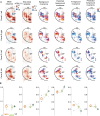
Figure 2.. Invariance to background sounds is hierarchically organized in ferret auditory cortex.

(A) Map of average response for an example hemisphere (ferret L). Responses are expressed in percent changes in cerebral blood volume (CBV) relative to baseline activity, measured in periods of silence. Values are averaged across depth to obtain this surface view of auditory cortex. (B) Map of test-retest reliability. In the following maps, only reliably responding voxels are displayed (test–retest > 0.3 for at least one category of sounds) and the transparency of surface bins in the maps is determined by the number of (reliable) voxels included in the average. (C) Map of considered regions of interest (ROIs), based on anatomical landmarks. The arrows indicate the example slices shown in (D) (orange: primary; green: non-primary example). (D) Responses to isolated and combined foregrounds. Bottom: responses to mixtures and foregrounds in isolation, for example, voxels (left: primary; right: non-primary). Each dot represents the voxel’s time-averaged response to every foreground (x-axis) and mixture (y-axis), averaged across two repetitions. r indicates the value of the Pearson correlation. Top: maps show invariance, defined as noise-corrected correlation between mixtures and foregrounds in isolation, for the example voxel’s slice with values overlaid on anatomical images representing baseline CBV. Example voxels are shown with white squares. (E) Map of background invariance for the same hemisphere (see Figure 2—figure supplement 2 for other ferrets). (F) Quantification of background invariance for each ROI. Colored circles indicate median values across all voxels of each ROI, across animals. Gray dots represent median values across the voxels of each ROI for each animal. The size of each dot is proportional to the number of voxels across which the median is taken. The thicker line corresponds to the example ferret L. ***: $p\le 0.001$ for comparing the average background invariance across animals for pairs of ROIs, obtained by a permutation test of voxel ROI labels within each animal. (G–I) Same as (D–F) for foreground invariance (comparing mixtures to backgrounds in isolation). AEG, anterior ectosylvian gyrus; MEG, medial ectosylvian gyrus; dPEG, dorsal posterior ectosylvian gyrus; VP, ventral posterior auditory field.

Figure 2—figure supplement 1.. Invariance dynamics.

For each voxel, we computed the Pearson correlation between the vectors of trial-averaged responses to mixtures and foregrounds (A) or backgrounds (B) with different lags. We then averaged these matrices across all responsive voxels to obtain the cross-correlation matrices shown here. The matrices here are not noise-corrected.

Figure 2—figure supplement 2.. Maps for all ferrets.

(A) Maps of mean response, test–retest reliability, true and predicted background and foreground invariance, for all recorded hemispheres. In the invariance maps, only reliable voxels are shown. (B) Comparison of metrics shown in (A) across primary (MEG) and non-primary regions (dPEG, VP), for voxels selected for prediction analyses (test-retest > 0 for each category, and > 0.3 for at least one category).

Figure 3.. Simple spectrotemporal tuning explains spatial organization of background invariance.

(A) Presentation of the two-stage filter-bank, or spectrotemporal model. Cochleagrams (shown for an example foreground and background) are convolved through a bank of spectrotemporal modulation filters. (B) Energy of foregrounds and backgrounds in spectrotemporal modulation space, averaged across all frequency bins. (C) Average difference of energy between foregrounds and backgrounds in the full acoustic feature space (frequency * temporal modulation * spectral modulation). (D) We predicted time-averaged voxel responses using sound features derived from the spectrotemporal model presented in (A) with ridge regression. For each voxel, we thus obtain a set of weights for frequency and spectrotemporal modulation features, as well as cross-validated predicted responses to all sounds. (E) Average model weights for MEG. (F) Maps of preferred frequency, temporal and spectral modulation based on the fit model. To calculate the preferred value for each feature, we marginalized the weight matrix over the two other dimensions. (G) Average differences of weights between voxels of each non-primary (dPEG and VP) and primary (MEG) region. (H) Background invariance (left) and foreground invariance (right) for voxels tuned to low (< 8 Hz) or high (> 8 Hz) temporal modulation rates within each region of interest (ROI). Colored circles indicate median value across all voxels of each ROI, across animals. Gray dots represent median values across the voxels of each ROI for each animal. **: $p\le 0.01$, ***: $p\le 0.001$ for comparing the average background invariance across animals for voxels tuned to low vs. high rates, obtained by a permutation test of tuning within each animal.

Figure 3—figure supplement 1.. Tuning to acoustic features for all ferrets.

Maps of preferred values for each dimension of acoustic space, obtained by marginalizing the fitted weight matrix over other dimensions.

Figure 4.. A model of auditory processing predicts hierarchical differences in ferret auditory cortex.

Same as in Figure 2 using cross-validated predictions from the spectrotemporal model. (A) Predicted responses to mixtures and foregrounds in isolation for example voxels (left: primary; right: non-primary). Each dot represents the voxel’s predicted response to foregrounds (x-axis) and mixtures (y-axis). r indicates the value of the Pearson correlation. Maps above show predicted invariance values for the example voxel’s slice overlaid on anatomical images representing baseline cerebral blood volume (CBV). Example voxels are shown with white squares. (B) Maps of predicted background invariance, defined as the correlation between predicted responses to mixtures and foregrounds in isolation. (C) Binned scatter plot representing predicted vs. measured background invariance across voxels. Each line corresponds to the median across voxels for one animal, using 0.1 bins of measured invariance. (D) Predicted background invariance for each region of interest (ROI). Colored circles indicate median value across all voxels of each ROI, across animals. Gray dots represent median values across the voxels of each ROI, for each animal. The size of each dot is proportional to the number of voxels across which the median is done. The thicker line corresponds to example ferret L. *: $p\le 0.05$; ***: $p\le 0.001$ for comparing the average predicted background invariance across animals for pairs of ROIs, obtained by a permutation test of voxel ROI labels within each animal. (E–H) Same as (A–D) for predicted foreground invariance, that is, comparing predicted responses to mixtures and backgrounds in isolation.

Figure 4—figure supplement 1.. Assessment and effect of model prediction accuracy across species.

(A) Map of model prediction accuracy (correlation between measured and cross-validated predicted responses) for the example ferret. (B) Histogram of prediction accuracy across voxels of each region, for ferrets. (C) Comparison of prediction accuracy vs. test–retest reliability across voxels. (D) Median predicted background invariance across voxels grouped in bins of observed prediction accuracy, in ferrets. Each thin line corresponds to the median across voxels within one subject for one region. Thick lines correspond to averages across subjects. (E). Same, for predicted foreground invariance. (F–I). Same as (B–E), for humans.

Figure 4—figure supplement 2.. Predicting from a model fitted on isolated sounds only.

(A) Predicted background invariance by region, with weights fitted using all sounds including mixtures (reproduced from Figure 4B). (B) Predicted background invariance by region, with weights fitted on the isolated sounds only (excluding mixtures). (C, D) Same as (A, B), for predicted foreground invariance. (E–H) Same as (A–D), for humans. *: $p\le 0.05$; ***: $p\le 0.001$.

Figure 5.. The spectrotemporal model is a poor predictor of human background invariance.

(A) We replicated our analyses with a dataset of a similar experiment measuring fMRI responses in human auditory cortex (Kell and McDermott, 2019). We compared responses in primary and non-primary auditory cortex, as delineated in Kell and McDermott, 2019. (B) Responses to mixtures and foregrounds in isolation for example voxels (left: primary; right: non-primary). Each dot represents the voxel’s response to foregrounds (x-axis) and mixtures (y-axis), averaged across repetitions. r indicates the value of the Pearson correlation. (C) Quantification of background invariance measured for each region of interest (ROI). Colored circles indicate median value across all voxels of each ROI, across subjects. Gray dots represent median values for each ROI and subject. The size of each dot is proportional to the number of (reliable) voxels across which the median is done. *:$p\le 0.05$; ***:$p\le 0.001$ for comparing the average predicted background invariance across subjects for pairs of ROIs, obtained by a permutation test of voxel ROI labels within each subject. (D) Binned scatter plot representing predicted vs measured background invariance across voxels. Each line corresponds to the median across voxels for one subject, using 0.1 bins of measured invariance. (D) Same as (C) for responses predicted from the spectrotemporal model. (F–I) Same as (B–E) for foreground invariance, that is, comparing predicted responses to mixtures and backgrounds in isolation.

Figure 5—figure supplement 1.. Spectrotemporal tuning properties for humans.

(A) Average difference of energy between foregrounds and backgrounds used in human experiments, in the acoustic feature space (frequency * temporal modulation * spectral modulation). (B) Average model weights for human primary auditory cortex. (C) Average differences of weights between voxels of human non-primary vs. primary auditory cortex.

Figure 5—figure supplement 2.. Invariance metrics are not affected by differences in test–retest reliability across regions.

(A) Background invariance across voxels grouped in bins of test–retest reliability (averaged across sound categories). (B) Same, for foreground invariance. Thin lines show the median across voxels within regions of interest (ROIs) of each animal. Thick lines show the median across voxels of an ROI, across all animals.

References

1. Bar-Yosef O, Nelken I. The effects of background noise on the neural responses to natural sounds in cat primary auditory cortex. Frontiers in Computational Neuroscience. 2007;1:3. doi: 10.3389/neuro.10.003.2007. - DOI - PMC - PubMed
1. Bimbard C, Demene C, Girard C, Radtke-Schuller S, Shamma S, Tanter M, Boubenec Y. Multi-scale mapping along the auditory hierarchy using high-resolution functional UltraSound in the awake ferret. eLife. 2018;7:e35028. doi: 10.7554/eLife.35028. - DOI - PMC - PubMed
1. Carruthers IM, Laplagne DA, Jaegle A, Briguglio JJ, Mwilambwe-Tshilobo L, Natan RG, Geffen MN. Emergence of invariant representation of vocalizations in the auditory cortex. Journal of Neurophysiology. 2015;114:2726–2740. doi: 10.1152/jn.00095.2015. - DOI - PMC - PubMed
1. Chi T, Ru P, Shamma SA. Multiresolution spectrotemporal analysis of complex sounds. The Journal of the Acoustical Society of America. 2005;118:887–906. doi: 10.1121/1.1945807. - DOI - PubMed
1. Christensen RK, Lindén H, Nakamura M, Barkat TR. White noise background improves tone discrimination by suppressing cortical tuning curves. Cell Reports. 2019;29:2041–2053. doi: 10.1016/j.celrep.2019.10.049. - DOI - PubMed
LinkOut - more resources