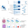
. 2025 Oct 8;16(1):8959.
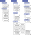
doi: 10.1038/s41467-025-64712-4.

Pathologist-like explainable AI for interpretable Gleason grading in prostate cancer

Gesa Mittmann #  1   2 Sara Laiouar-Pedari #  1 Hendrik A Mehrtens #  1 Sarah Haggenmüller  1 Tabea-Clara Bucher  1 Tirtha Chanda  1   2 Nadine T Gaisa  3   4 Mathias Wagner  5 Gilbert Georg Klamminger  5 Tilman T Rau  6 Christina Neppl  6 Eva Maria Compérat  7 Andreas Gocht  8 Monika Haemmerle  9 Niels J Rupp  10   11 Jula Westhoff  12 Irene Krücken  13   14 Maximilian Seidl  6 Christian M Schürch  15   16 Marcus Bauer  9 Wiebke Solass  17 Yu Chun Tam  18 Florian Weber  19 Rainer Grobholz  11   20 Jaroslaw Augustyniak  21 Thomas Kalinski  22 Christian Hörner  23 Kirsten D Mertz  24   25 Constanze Döring  26 Andreas Erbersdobler  27 Gabriele Deubler  28 Felix Bremmer  29 Ulrich Sommer  30 Michael Brodhun  31 Jon Griffin  32 Maria Sarah L Lenon  33   34 Kiril Trpkov  35 Liang Cheng  36 Fei Chen  37 Angelique Levi  38 Guoping Cai  38 Tri Q Nguyen  39 Ali Amin  40 Alessia Cimadamore  41 Ahmed Shabaik  42 Varsha Manucha  43 Nazeel Ahmad  44 Nidia Messias  45 Francesca Sanguedolce  46 Diana Taheri  47   48 Ezra Baraban  49 Liwei Jia  50 Rajal B Shah  50 Farshid Siadat  35 Nicole Swarbrick  51   52 Kyung Park  37 Oudai Hassan  53 Siamak Sakhaie  54 Michelle R Downes  55 Hiroshi Miyamoto  56 Sean R Williamson  57 Tim Holland-Letz  58 Christoph Wies  1   2 Carolin V Schneider  59 Jakob Nikolas Kather  60   61   62   63 Yuri Tolkach  64   65 Titus J Brinker  66
Affiliations

Pathologist-like explainable AI for interpretable Gleason grading in prostate cancer

Gesa Mittmann et al. Nat Commun. .

Abstract

The aggressiveness of prostate cancer is primarily assessed from histopathological data using the Gleason scoring system. Conventional artificial intelligence (AI) approaches can predict Gleason scores, but often lack explainability, which may limit clinical acceptance. Here, we present an alternative, inherently explainable AI that circumvents the need for post-hoc explainability methods. The model was trained on 1,015 tissue microarray core images, annotated with detailed pattern descriptions by 54 international pathologists following standardized guidelines. It uses pathologist-defined terminology and was trained using soft labels to capture data uncertainty. This approach enables robust Gleason pattern segmentation despite high interobserver variability. The model achieved comparable or superior performance to direct Gleason pattern segmentation (Dice score: 0.713 ± 0.003 vs. 0.691 ± 0.010 ) while providing interpretable outputs. We release this dataset to encourage further research on segmentation in medical tasks with high subjectivity and to deepen insights into pathologists' reasoning.


Conflict of interest statement

Competing interests: TJB owns a company that develops mobile apps (Smart Health Heidelberg GmbH, Heidelberg, Germany). TJB received honoraria from Novartis, Roche and HEINE Optotechnik. JNK declares consulting services for Panakeia, AstraZeneca, MultiplexDx, Mindpeak, Owkin, DoMore Diagnostics, and Bioptimus. Furthermore, he holds shares in StratifAI, Synagen, Tremont AI, and Ignition Labs, has received an institutional research grant from GSK, and has received honoraria from AstraZeneca, Bayer, Daiichi Sankyo, Eisai, Janssen, Merck, MSD, BMS, Roche, Pfizer, and Fresenius. YT declares consulting services for Indica Labs, AstraZeneca, MSD, Pfizer; royalties not related to this study (Indica Labs). CMS is a cofounder and shareholder of Vicinity Bio GmbH, and is a scientific advisor to and has received research funding from Enable Medicine Inc., all outside the current work. HM declares consulting services for PathXL, Invicro, and PathAI, outside of this work. NJR discloses an advisory board function for AbbVie AG, and receipt of a travel grant from Roche Diagnostics, both outside of the scope of the current work. IK has received honoraria from AstraZeneca and Menarini Stemline, as well as gifts/financial advantages from Roche (conference invitations). NTG received an institutional research grant from Janssen/Johnson & Johnson and declares consulting services for/honoraria from AstraZeneca, Janssen, Merck, BMS, Daiichi Sankyo, and Bayer. No other conflicts of interest are declared by any of the authors.

Figures

Fig. 1
Fig. 1. Overview.
a We developed GleasonXAI, a U-Net model that predicts the presence of histological features closely aligned with the pathologists’ consensus. Due to training with soft labels, the predicted distribution often reflects the agreement of the annotators. b In the annotation process, up to six pathologists evaluated the TMA core images, identifying areas for each Gleason pattern, which were then merged using the simultaneous truth and performance level estimation (STAPLE) algorithm. Subsequently, three pathologists independently annotated histologic patterns based on a predefined ontology. We compared training on two labeling approaches: soft and hard labels. In the soft label approach, each pixel is represented as a distribution across the annotated classes, while the hard label method assigns a class to each pixel through majority voting. Further details on post- and pre-processing, such as the masking of background pixels, can be found in the Methods section. Created in bioRender.com.
Fig. 2
Fig. 2. Class distribution.
Number of TMA core images with at least one occurrence of a the specified Gleason pattern, b the specified explanation, and c the specified sub-explanation. Benign tissue is not included, as it is present in all images. A mapping of sub-explanation numbers to text and is available in Supplementary Tables 1 to 3. The mapping of the explanations to their long version is available in the Methods. Colors of sub-explanations in (c) map to the colors of their parent explanation in (b). All green colors map to Gleason pattern 3, blue colors to Gleason pattern 4, and red colors to Gleason pattern 5. Source data are provided as a Source Data file.
Fig. 3
Fig. 3. Agreement of annotators for explanations on the image-level.
a Confusion matrix between the Gleason score presented to the annotators and Gleason pattern of the applied explanations in the images (Each Gleason pattern was counted only once per image, regardless of number of agreeing pathologists), and b heatmap containing the number of TMA core images in which n out of the three annotators indicated the presence of the Gleason pattern (left, top) and explanations (left, bottom), and the resulting Fleiss’ kappa within groups of three raters (on the right) as boxplot. In the boxplot, dots represent the Fleiss’ kappa value of a group of n=3 annotators. Boxes represent the inter-quartile range, with the centre line marking the median, the white diamonds mark the mean value, and whiskers extend to the minimum and maximum within 1.5 of the inter-quartile range. For most Gleason patterns and explanations, the Fleiss’ kappa values of 14 groups of annotators are included. As not every group used all categories, the number of groups taken into account is reduced for glomeruloid glands (13 groups), single cells (13 groups), and comedonecrosis (11 groups). Precise numerical values can be found in Supplementary Tables 8 to 10, and the figure for sub-explanations in Supplementary Fig. 1. The mapping of the explanations to their long version is available in the Methods. Exemplary differences in the consensus of the three annotators are shown in (c) with an example for high agreement in the first row and an example for labels with low class agreement in the bottom row. The scale bar corresponds to 200 µm. Source data are provided as a Source Data file.
Fig. 4
Fig. 4. Agreement of annotators for explanations on pixel-level.
Agreement demonstrated by a the proportion of pixels annotated for a given class by at least one annotator, stratified by the number of annotators indicating the presence of the explanation and b the percentage of foreground pixels annotated with an explanation by at least one annotator. The mapping of the explanations to their long version is available in the Methods.
Fig. 5
Fig. 5. Results.
Results for our models trained with different loss functions, evaluated on the Gleason patterns and the corresponding explanations. Using our ontology, we mapped the labels upwards, allowing a comparison between the models trained on the explanations with those directly trained on the Gleason patterns. The bar plots display both the mean and the standard deviation of three models trained with different seeds but the same hyperparameters, with the mean values additionally indicated within the bars. The result of the n = 3 technical replicates are indicated as dots. The green bar charts represent metrics for the hard label approaches, while the blue bars correspond to the soft label approaches. For the Dice metrics, higher values indicate better performance, while for the L1-norm, lower values are preferable. Source data are provided as a Source Data file.
Fig. 6
Fig. 6. Comparison between GleasonXAI predictions and pathologist’s annotations.
Comparison described by a proportion of predicted probability mass for each explanation, compared to the soft-label probability mass and the proportion of pixels with a majority vote for an explanation compared to the number of pixels with an argmax prediction for this explanation, and b the confusion matrix for the argmax prediction and the majority label, presented in percentages of pixels. The gray boxes highlight the explanations corresponding to a common Gleason pattern. For a more comprehensible representation, c illustrates the confusion matrix in percentage when the explanations were mapped to Gleason patterns. The mapping of the explanations to their long version is available in the Methods.
Fig. 7
Fig. 7. Result Visualization.
Visualization of examples of segmentation results for the GleasonXAI model compared to the three pathologists’ annotations. The segmentation images depict the argmax of the per-pixel distribution for the predictions of the model. a, b showcase examples of high agreement between the three annotators and the model. cg highlight cases with greater disagreement among the three annotators, where the segmentation maps of the model often fell between the annotators’ interpretations, reflecting the training objective of our soft-label approach. h, i illustrate instances of strong disagreement between the model and the annotators. Green labels belong to Gleason pattern 3, blue to Gleason pattern 4 and red to Gleason pattern 5. The mapping of the explanations to their long version is available in the Methods. The scale bar corresponds to 200 µm.
Fig. 8
Fig. 8. Overview of the explanatory Gleason pattern ontology.
Generic terms based on the WHO and ISUP2014 guidelines summarize the explanations corresponding to our initial ontology version. As the term “hypernephroid pattern” is now discouraged, we replaced it with “poorly formed lumens, cells with clear cytoplasm lying next to each other without true definition of the gland”. Gleason pattern classes are marked in dark blue, explanation classes in light blue, and sub-explanations in white. For our figures, we use shortened names of the explanations, which are shown in square brackets for explanations, and in the numbering in the bottom right for the sub-explanations.

References

    1. Ferlay, J. et al. Cancer statistics for the year 2020: An overview. Int. J. Cancer149, 778–789 (2021). - PubMed
    1. Gleason, D. F., Mellinger, G. T. & Veterans Administration Cooperative Urological Research Group Prediction of Prognosis for Prostatic Adenocarcinoma by Combined Histological Grading and Clinical Staging. J. Urol.197, 134–139 (1974). - PubMed
    1. van Leenders, G. J. L. H. et al. The 2019 International Society of Urological Pathology (ISUP) Consensus Conference on Grading of Prostatic Carcinoma. Am. J. Surg. Pathol.44, e87 (2020). - PMC - PubMed
    1. Epstein, J. I. et al. The 2019 Genitourinary Pathology Society (GUPS) White Paper on Contemporary Grading of Prostate Cancer. Arch. Pathol. Lab. Med.145, 461–493 (2021). - PubMed
    1. Leitlinienprogramm Onkologie (Deutsche Krebsgesellschaft, Deutsche Krebshilfe, AWMF). S3-Leitlinie Prostatakarzinom, Langversion 7.0. AWMF Leitlinienregister. Registernummer 043-022OL. https://www.leitlinienprogramm-onkologie.de/leitlinien/prostatakarzinom/ (2024).