Statistical Inference for the Evolutionary History of Cancer Genomes

Abstract

Recent years have seen considerable work on inference about cancer evolution from mutations identified in cancer samples. Much of the modeling work has been based on classical models of population genetics, generalized to accommodate time-varying cell population size. Reverse-time, genealogical views of such models, commonly known as coalescents, have been used to infer aspects of the past of growing populations. Another approach is to use branching processes, the simplest scenario being the classical linear birth-death process. Inference from evolutionary models of DNA often exploits summary statistics of the sequence data, a common one being the so-called Site Frequency Spectrum (SFS). In a bulk tumor sequencing experiment, we can estimate for each site at which a novel somatic point mutation has arisen, the proportion of cells that carry that mutation. These numbers are then grouped into collections of sites which have similar mutant fractions. We examine how the SFS based on birth-death processes differs from those based on the coalescent model. This may stem from the different sampling mechanisms in the two approaches. However, we also show that despite this, they are quantitatively comparable for the range of parameters typical for tumor cell populations. We also present a model of tumor evolution with selective sweeps, and demonstrate how it may help in understanding the history of a tumor as well as the influence of data pre-processing. We illustrate the theory with applications to several examples from The Cancer Genome Atlas tumors.

Keywords: Cancer evolution; birth-death processes; bulk sequencing; clonal selection; coalescents; ploidy; site frequency spectrum; tumor heterogeneity.

Fig. 1.

Left panel: Genealogy of a sample of n = 20 cells includes 13 mutational events, denoted by black dots. Mutations 4, 5, 7, 10, 11, 12, and 13 (total of 7 mutations) are present in a single cell, mutations 1, 2, and 3 (total of 3 mutations) are present in three cells, mutations 8 and 9 (2 mutations) are present in six cells, and mutation 6 (1 mutation) is present in 17 cells. Right panel: The observed site frequency spectrum, $S_{20}\left(1\right)=7,S_{20}\left(3\right)=3,S_{20}\left(6\right)=2$, and $S_{20}\left(17\right)=1$, other values equal to 0.

Fig. 2.

Numerical example of the expected SFS for the lbdp (semi-logarithmic scale). Continuous line: expected $\mathbb{E}{S}_n(k)$ (interpolated for visual convenience); circles: corresponding average of 10,000 simulations; dashes: standard deviation estimate based on 10,000 simulations; dotted line, diamonds and triangles: median and first and third quartile of 10,000 simulations. The parameters for this simulation (cf. Table 2) are $n=p\mathbb{E}N(t)=30,r=1,\theta =1,\alpha =0.999999,t=100$ for simulations, $t=\mathrm{\infty }$ for $\mathbb{E}{S}_n(k)$. Other parameters can be calculated from these.

Fig. 3.

Comparison of expected SFS based on the hypergeometric formula (8) with parameters as in Table 1 (dotted lines), Griffiths–Tavaré theory (continuous lines), and Durrett’s approximation (dashed lines). Three cases as in Table 1, fast-growing tumors (red), moderate – growing (blue), and slow growing ones (black) are considered. $\theta =1$ has been assumed. Unscaled parameters listed in Table 1, can be converted to scaled ones, using Table 2.

Fig. 4.

Expected SFS based on the hypergeometric formula (8) with parameters as for the center scenario in Table 1, that is, $N={10}^7,n=30$ and $r=0.04029$, but with $1-\alpha ={10}^{-8},{10}^{-6},0.0001,0.01,0.1,0.5$ (dashed, dotted, continuous, and again dashed, dotted and continuous lines), and $\theta =1$, compared to GT SFS (diamonds) and Durrett approximation (circles) with matching parameters. Unscaled parameters listed here, can be converted to scaled ones, using Table 2.

Fig. 5.

Events in the tumor evolution model. Horizontal intervals denote genomes with mutations denoted as $\times -s$. At time $t_0=0$, the initial cell population (clone 0) arises, grows at rate ${\gamma }_0$, and mutates at rate ${\theta }_0$ per time unit per genome (blue arrows). At time $t_1>0$, a secondary sub-clone 1 arises (red arrow), which grows at rate ${\gamma }_1$ and mutates at rate ${\theta }_1$ (yellow arrows). The new clone arises on the background of a haplotype of $K$ mutations (denoted by dots on the genome). At time $t_2>t_1>0$, the tumor is diagnosed and a sample of DNA is sequenced.

Fig. 6.

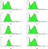
Fitting the SFS of case TCGA-AA-3977 (colon cancer). The theoretical SFS (red lines, Eqn. (14)) is fitted to the patient’s SFS (green bars). The blue and black dotted lines denote the contribution of the neutral part and sub-clones in the fitted SFS, respectively. Threshold combinations of variant and total read counts: $\left[A\right]:L=5,M=0$, $\left[B\right]:L=10,M=0$, $\left[C\right]:L=15,M=0$, $\left[D\right]:L=20,M=0$, $\left[E\right]:L=5,M=20$, $\left[F\right]:L=5,M=30$, $\left[G\right]:L=5,M=40$, $\left[H\right]:L=5,M=50$.

Fig. 7.

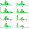
Fitting the SFS of case TCGA-86-A4D0 (lung cancer). The theoretical SFS (red lines, Eqn. (14)) is fitted to the patient’s SFS (green bars). The blue and black dotted lines denote the contribution of the neutral part and sub-clones in the fitted SFS, respectively. Driver mutations are denoted in blue at their frequencies. Threshold combinations of variant and total read counts: $\left[A\right]:L=5,M=0$. $\left[B\right]:L=10,M=0$. $\left[C\right]:L=15,M=0$. $\left[D\right]:L=20,M=0$. $\left[E\right]:L=5,M=20$. $\left[F\right]:L=5,M=50$. $\left[G\right]:L=5,M=80$. $\left[H\right]:L=5,M=100$.

Fig. 8.

[A]: Example of a simulated tree and resulting SFS. The y-axis is time, x-axis includes invisible indices of cells such that progeny of any given cell is grouped together. The three types of mutations correspond to the SFS. [B]: the SFS resulting from sampling the simulation under the TCGA distribution.

Fig. 9.

The choice of sampling distribution distorts the resulting SFS. [A]: the simplified presentation of the simulated tree. [B, C, D]: the SFS resulting from sampling the simulation under the binomial distribution with mean 50 (B), 80 (C) and 150 (D). [E]: PDF of the TCGA sampling distribution. [F]: the SFS resulting from sampling from the simulated tree according to the TCGA distribution. Parameters: $T=1000,s=800,b=0.0162,b^{⊛}=0.0721,d=d^{⊛}=0.01,\theta =1$.

References

1. Abramowitz M and Stegun IA (1964). Handbook of Mathematical Functions. Applied Mathematics Series 55. National Bureau of Standards.
1. Cheek D and Antal T (2018). Mutation frequencies in a birth-death branching process. Ann. Appl. Probab. 28 3922–3947. MR3861830 10.1214/18-AAP1413 - DOI
1. Del Monte U (2009). Does the cell number 109 still really fit one gram of tumor tissue? Cell Cycle 8 505–506. 10.4161/cc.8.3.7608 - DOI - PubMed
1. Dinh KN, Jaksik R, Kimmel M, Lambert A and Tavaré S (2020). Supplement to “Statistical inference for the evolutionary history of cancer genomes.” 10.1214/19-STS7561SUPP. - DOI
1. Durrett R (2013). Population genetics of neutral mutations in exponentially growing cancer cell populations. Ann. Appl. Probab. 23 230–250. MR3059234 10.1214/11-AAP824 - DOI - PMC - PubMed
LinkOut - more resources