Improved reconstruction of single-cell developmental potential with CytoTRACE 2

Abstract

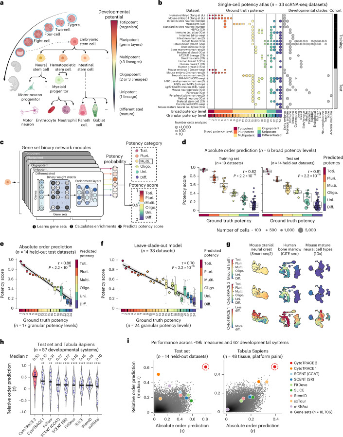
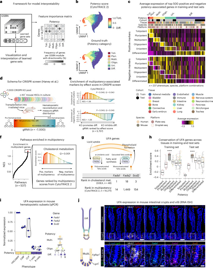
While single-cell RNA sequencing has advanced our understanding of cell fate, identifying molecular hallmarks of potency-a cell's ability to differentiate into other cell types-remains a challenge. Here we introduce CytoTRACE 2, an interpretable deep learning framework for predicting absolute developmental potential from single-cell RNA sequencing data. Across diverse platforms and tissues, CytoTRACE 2 outperformed previous methods in predicting developmental hierarchies, enabling detailed mapping of single-cell differentiation landscapes and expanding insights into cell potency.

Fig. 1. Development and benchmarking of CytoTRACE 2.

a, Overview of cell potency across six developmental categories. b, Summary of the 33-dataset single-cell potency atlas. c, Schematic of the CytoTRACE 2 model. Toti., totipotent; Pluri., pluripotent; Multi., multipotent; Oligo., oligopotent; Uni., unipotent; Diff., differentiated. d, CytoTRACE 2 performance across six broad potency categories in training and held-out test sets, with mean potency scores shown for each standardized phenotype–dataset pair (circles). e, CytoTRACE 2 performance across 17 evaluable granular potency levels in held-out test data. Points denote mean potency score per phenotype; large circles indicate the median across these points for each granular potency level. Thick black lines (x axis) separate broad potency categories. A linear regression line with 95% confidence band is shown. f, Same as e, but using a leave-clade-out strategy, where each of 19 developmentally distinct clades (b) was held out during training. For d–f, concordance with ground truth was assessed using weighted Kendall correlation (τ) applied to single cells, with significance assessed by two-sided z-test. Box plots show medians, quartiles and 1.5 × interquartile range (IQR). g, Uniform Manifold Approximation and Projection (UMAP) of three held-out datasets showing ground truth (top), CytoTRACE 2 (middle) and CytoTRACE 1 (bottom). h, Violin plots comparing nine methods for reconstructing 57 developmental systems. P values were calculated by two-sided Wilcoxon tests against CytoTRACE 2; **P < 0.01; ****P < 0.0001. i, Performance comparison with eight previous methods and 18,706 gene sets in the test set (left) and Tabula Sapiens (right) using weighted τ to assess absolute (six broad potency levels) and relative order (median correlation across individual trajectories). a and c were created using BioRender.com.

Fig. 2. Model interpretability and cross-tissue signatures of cell potency.

a, Schematic for characterizing CytoTRACE 2 gene sets and feature importance. b, UMAP of gene set expression levels in training–test sets, aggregated in a 0.5 × 0.5 grid, colored by CytoTRACE 2 (top) or ground truth potency (bottom). c, Expression of top 500 positive (pos.) and negative (neg.) markers per potency category, shown across 237 pseudo-bulks aggregated by phenotype, species and platform from training–test sets. d, Overview of a CRISPR knockout (KO) screen assessing in vivo differentiation effects in hematopoietic stem cells (HSCs). e, Enrichment of top CytoTRACE 2 multipotency markers among genes whose knockout promotes or inhibits HSC differentiation (from d), using GSEA. f, GSEA of 537 pathways in genes ranked by multipotency scores, highlighting ‘cholesterol metabolism’. g, Top: overview of UFA pathways, inspired by ref. . Bottom: top UFA biosynthesis genes (Fads1, Fads2 and Scd2) ranked by GSEA and CytoTRACE 2 multipotency scores). h, Single-sample GSEA of UFA genes across 237 pseudo-bulk samples, colored by tissue type as in c. ****P < 0.0001 (one-sided permutation testing). Box plots show medians, quartiles and 1.5 × IQR. i, qPCR of UFA genes in FACS-purified mouse hematopoietic subsets (n = 3), normalized to HSC/MPP; Actb as internal control. MPP, multipotent progenitor; CMP, common myeloid progenitor; CLP, common lymphoid progenitor. Violin plots show median and range. j, In situ mRNA imaging of mouse jejunum (top) shows spatial expression of multipotent (Lgr5 and Fgfbp1), proliferation (Mki67), and UFA (Fads1, Fads2 and Scd2) marker genes in crypts and villi. Higher magnification views (bottom) highlight boxed regions. Cell boundaries were visualized with E-cadherin immunostaining; asterisks mark representative Lgr5⁺ crypt base columnar (CBC) cells. TA, transit-amplifying. Scale bars, 50 μm (top), 10 μm (bottom). Images are representative of three mice. Images in a, d, g, i, j were created using BioRender.com. NES, normalized enrichment score.

Extended Data Fig. 1. CytoTRACE 2 architecture and benchmarking metrics.

a, Schematic overview of the CytoTRACE 2 core model, focusing on architectural details and key operations between the input layer and output layer for a single gene set binary network (GSBN) module. Note that six GSBN modules, one per broad potency category, are included in the full model, as illustrated in Fig. 1c. For additional details, see Methods. b, Serial impact of three postprocessing procedures (“Postprocessing” in Methods) on the accuracy of predicting (i) relative developmental orderings (n = 33 systems; bottom) and (ii) potency classes (F1 score, mean-aggregated across six broad potency categories; top) on training datasets (Methods). All results were obtained via leave-one-out cross-validation (LOOCV). c, Box plot showing the performance of CytoTRACE 2 for the prediction of relative orderings (Supplementary Table 4) after subsampling cells for the Markov diffusion step of the postprocessing procedure (Methods). All training datasets were analyzed using LOOCV (Supplementary Table 1). d, Illustration of the difference between absolute and relative developmental potential using two hypothetical scRNA-seq datasets, one spanning totipotent through pluripotent cells (‘Embryo’) and the other encompassing multipotent through differentiated cells (‘Blood’). Hypothetical prediction scores are shown for absolute and relative orderings, with the latter reset for each dataset (for example, as for CytoTRACE 1, RNA velocity, Monocle, and CellRank). ESC, embryonic stem cell; HSC, hematopoietic stem cell; CMP, common myeloid progenitor; CLP, common lymphoid progenitor; MkE, megakaryocyte-erythroid progenitor; GM, granulocyte progenitor; B-p, B cell progenitor; T-p, T cell progenitor; Mk, megakaryocyte; E, erythrocyte; G, granulocyte; M, monocyte. e-f, Impact of hyperparameter values on training set performance, showing weighted accuracy for single-cell potency classification using nested LOOCV (Supplementary Table 6; Methods). e, Left: Each point (n = 500) denotes the results from one iteration of the hyperparameter sweep. Right: Same as the left but showing weighted accuracy plotted by the number of gene sets per GSBN module. f, Weighted accuracy of models trained using distinct gene set enrichment procedures (AMS and/or UCell) after selecting robust hyperparameter values as described in Methods. Statistical significance was determined using a two-sided paired Wilcoxon test in panels b and c and a two-sided unpaired Wilcoxon test in panel f. *P < 0.05; **P < 0.01; ***P < 0.001; ****P < 0.0001; ns, not significant. Note that tissue-specific expression matrices from plate- and droplet-based platforms within Tabula Muris were analyzed individually in panels b and c for clarity, yielding 33 total systems with known developmental orderings. In b, c, e, and f, the box center lines, bounds of the box, and whiskers denote medians, 1st and 3rd quartiles, and minimum and maximum values within 1.5 × IQR (interquartile range) of the box limits, respectively. Panel a was created using BioRender.com.

Extended Data Fig. 2. Validation and generalizability of CytoTRACE 2.

a, Performance of CytoTRACE 2 for reconstructing relative developmental trajectories (left) and six broad potency categories (right) in 33 ground truth scRNA-seq datasets (Fig. 1b), stratified by species and platform. Performance was evaluated at the single-cell level using weighted Kendall correlation (τ), as described in Supplementary Table 5 and Methods. To promote a fair comparison, we evaluated absolute order correlations (right) with and without the inclusion of totipotent and pluripotent cells, as the corresponding potency categories were not available for human and droplet-only datasets in the test cohort. ns, not significant (two-sided unpaired Wilcoxon test). b, Same as panel a (left) but showing relative order performance stratified by developmental clade (Fig. 1b). ns, not significant (Kruskal-Wallis test). c, Same as Fig. 1d-e but showing performance on 21 cell phenotypes that were unseen during model training, including cranial neural crest cells, apical progenitors, skeletal stem cells, epsilon cells, and photoreceptor cells (Supplementary Table 7). d, Performance of CytoTRACE 2 on different training-test configurations, comparing the original split (‘Original test set’; Fig. 1b) with three additional splits, the latter of which were randomized to balance potency categories between cohorts (Supplementary Table 8; Methods). Performance was evaluated with four metrics, each calculated at the single-cell level in held-out data: absolute order (weighted τ), relative order (median weighted τ across evaluable systems with known developmental orderings), multiclass F1 for predicting broad potency classes (n = 6), and one minus the mean absolute error (MAE) for predicting broad potency classes (n = 6). For details, see Methods. e, Same as Fig. 1e but showing held-out data from three random training/test splits in d. In a-e, the box center lines (a-d) and circles (c right and e), bounds of the box, and whiskers denote medians, 1st and 3rd quartiles, and minimum and maximum values within 1.5 × IQR (interquartile range) of the box limits, respectively.

Extended Data Fig. 3. Robustness of CytoTRACE 2.

a-c, Impact of perturbing potency labels in the training set. a, Heat maps depicting individual potency labels and their transition probabilities at different perturbation levels (Methods). b-c, Performance of CytoTRACE 2 models trained on potency labels with defined perturbation levels (as illustrated in a and described in Methods) applied to individual cells (b) or phenotypes (c) in the training set. Performance in held-out test data was evaluated with four metrics: absolute order (weighted τ of broad potency levels across datasets), relative order (median weighted τ of each dataset analyzed individually), multiclass F1 for predicting broad potency classes (n = 6), and the mean absolute error (MAE) for predicting broad potency classes (n = 6). For details, see Methods. Absolute order (τ), relative order (τ), and F1 score are expressed as a percentage of the results obtained with the unperturbed CytoTRACE 2 model. Each point represents the mean across five replicates of random perturbation. Error bars represent 95% confidence intervals. d, Analysis of robustness to the number of genes per cell using all test datasets (n = 14) (Supplementary Table 1) assessed with the same metrics as panels b and c. Results for each dataset represent the average across five rounds of gene count downsampling and are expressed relative to results with no downsampling. e, Same as panel d but shown for UMIs per cell in evaluable test datasets (n = 7). f, Impact of the number of cells per phenotype on the consistency of CytoTRACE 2 potency scores in test datasets. Eleven phenotypes spanning a range of potencies were titrated in defined amounts (x-axis) while other cells were left unchanged. CytoTRACE 2 was then applied to predict potency scores. Points represent averages from five random samplings (without replacement) per phenotype and error bars represent 95% confidence intervals.

Extended Data Fig. 4. CytoTRACE 2 correctly identifies a transient pluripotent cell state during mouse cranial neural crest development.

Same as Fig. 1g but focusing on mouse cranial neural crest cells profiled by Zalc et al.. Left inset: Log expression levels of core pluripotency factor Pou5f1 in mouse cranial neural crest cells (CNCCs). Right inset: Cells predicted as pluripotent by CytoTRACE 2. Cells predicted as pluripotent by CytoTRACE 2 showed significantly higher Pou5f1 expression than others, with P = 2.6 × 10⁻⁵ by two-sided Wilcoxon test.

Extended Data Fig. 5. Large-scale reconstruction of cell potency during mouse embryogenesis.

a, Overview of single-cell expression datasets analyzed in b-e and corresponding developmental time points profiled (n = 62). Icons denoting key stages of mouse embryogenesis were created using BioRender.com. b, Linearity between the average CytoTRACE 2 potency score per time point (weighted equally across author-annotated phenotypes) expressed in rank space (y-axis) and the corresponding time points (n = 62; x-axis). Concordance was calculated using linear regression (dashed line) and Kendall correlation (τ), with the latter weighted by the number of time points per embryonic day. c, Scatter plot comparing the performance of CytoTRACE 2 to previous approaches for reconstructing the temporal hierarchy of 45 time points spanning organogenesis (beginning at E8.0) to birth (y-axis) versus 17 time points preceding organogenesis (x-axis). Correlations are weighted by whole day intervals to account for imbalances in the number of evaluable time points per day. Point sizes represent the average weighted Kendall correlation per approach. d, Top: Data-driven lineage tree of mouse embryogenesis, where nodes represent cell types (n = 259), edges represent developmental transitions inferred by Qiu et al., and colors represent the corresponding rank distance from each cell type to the root (“Ground truth”). Center and bottom: Same as top, but with CytoTRACE 2 and CytoTRACE 1 predictions each averaged by phenotype, then rank-ordered along the path to the root. Lower ranks indicate shorter distances. Distances were averaged for cell types with multiple direct paths to the root. e, Scatter plots showing all distances in d, with concordance between CytoTRACE methods (center and bottom panels of d) and lineages inferred by Qiu et al. (top panel of d). The significance of τ in b and e was determined using a two-sided Z-test.

Extended Data Fig. 6. Tracing developmental lineages in AML and oligodendroglioma.

a, Box plots showing relative expression levels of cell state signatures from patients with acute myeloid leukemia (AML) in 13,445 AML cells stratified by potency categories identified by CytoTRACE 2. Each point denotes a single gene from the corresponding gene set ID indicated above the plot (Supplementary Table 10). Genes were internally normalized within each tumor sample as the mean log₂ fold change (FC) within a given potency category versus the remaining cells in the tumor, as described in Methods, then z-score normalized (standardized) across potency categories. The four signatures, LSPC-Primed, LSPC-Quiescent, GMP-like, and Mono-like, are expected to be most highly expressed in multipotent, multipotent, oligopotent, and unipotent/differentiated cells, respectively (Supplementary Table 10). Statistical significance comparing the expected potency level(s) with each other potency level was determined by a two-sided Wilcoxon test. ****P < 0.0001. Box center lines, bounds of the box, and whiskers denote medians, 1st and 3rd quartiles, and minimum and maximum values within 1.5 × IQR (interquartile range) of the box limits, respectively. b, Left: Scatter plot of oligodendroglioma cells from six tumors organized by previously described stemness and lineage enrichment scores. Right: Stacked bar plot showing how the fractional representation of cells with predicted potency categories (CytoTRACE 2) changes as a function of author-supplied stemness scores (y-axis). Cells predicted to have the highest oligo- and multilineage potential by CytoTRACE 2 correspond to those annotated as stem-like by Tirosh et al.. Potency colors reflect eight evenly spaced bins per potency category.

Extended Data Fig. 7. Benchmarking against supervised machine learning methods.

a, Box plots comparing the performance of CytoTRACE 2 against eight baseline methods (supervised machine learning models, including leading tools for reference-guided annotation of scRNA-seq data) implemented for single-cell potency classification (Methods). Each method was trained to assign cells to six broad potency categories using identical training-test splits. Four-fold cross-validation was performed for each method, where each point represents performance in one fold of held-out data (the original training-test split [Fig. 1b] and three random splits [Supplementary Table 8]). Performance was assessed at the single-cell level using multiclass F1 (left) and one minus the mean absolute error (MAE; right) for predicting broad potency classes (n = 6). Box center lines, bounds of the box, and whiskers denote medians, 1st and 3rd quartiles, and minimum and maximum values within 1.5 × IQR (interquartile range) of the box limits, respectively. b, Scatter plot comparing median performance scores for all methods from panel a.

Extended Data Fig. 8. Benchmarking against scVelo.

a-b, Representative test datasets comparing CytoTRACE 2 and scVelo. a, UMAP representation of mouse pancreas development (10x) (Supplementary Table 1). Left: Cells colored by ground truth granular potency level (Fig. 1b; Supplementary Table 3). Center: Cells colored by CytoTRACE 2 potency scores. Right: Cells colored by scVelo latent time (differential kinetics model). b, Same as a but showing human bone marrow (CITE-seq) (Supplementary Table 1). c, Left: Bar plot showing mean absolute order (weighted τ applied to single cells) performance across six broad potency levels (circles) and ten granular order potency levels (triangles) for nine test datasets evaluable by CytoTRACE 2 and scVelo (Supplementary Tables 3 and 14; Methods). Two models are shown for the latter: dynamical latent time and differential kinetics latent time. Right: Violin and box plots showing relative order performance (weighted τ applied to single cells) on the same test datasets (n = 8 evaluable datasets with relative developmental orderings, Supplementary Tables 4 and 14). Statistical significance was determined by two-sided paired t test. Violin plot bounds denote minimum and maximum values. Box center lines, bounds of the box, and whiskers denote medians, 1st and 3rd quartiles, and minimum and maximum values within 1.5 × IQR (interquartile range) of the box limits, respectively. d, Same as Fig. 1e but shown for the nine evaluable test datasets in c. Left: CytoTRACE 2 potency scores. Right: scVelo latent time (differential kinetics model). Statistical significance was determined using a one-sided Z-test. ns, not significant.

Extended Data Fig. 9. Extended analysis of potency programs and genes.

a, Same as Fig. 2b but separated by cohort, species, cellular system (three general categories shown for clarity), and scRNA-seq platform. The embedding in Fig. 2b is shown as a reference in the upper left. Colors denote potency scores (same as the color bar in Fig. 2b, top) for reference and cohort-stratified embeddings. b, Heat map depicting pairwise similarity of gene sets learned by CytoTRACE 2 across all 19 ensemble models from leave-one-out cross-validation on the 19-dataset training cohort. Overlap was quantified by Jaccard index and stratified into gene sets with positive (left, n = 1,490) and negative weights (right, n = 1,246); gene set polarity was determined as described in “Interpretability,” Methods. c, Same as Fig. 2e but showing the consistency between CytoTRACE 2 multipotency markers and hematopoietic stem cell (HSC) knockout (KO) phenotypes across a range of top $k$ markers, whether positive or negatively associated with multipotency ($k$ = 50, 100, 200, and 500). GSEA statistics are expressed as directed –log₁₀ Q values. Statistical significance between groups was determined using a two-sided unpaired Wilcoxon test. Box center lines, bounds of the box, and whiskers denote medians, 1st and 3rd quartiles, and minimum and maximum values within 1.5 × IQR (interquartile range) of the box limits, respectively. d, Same as c, but showing the median directed –log₁₀ Q value across all top $k$ markers shown in c, stratified by positive and negative markers, and extended to all potency categories in the CytoTRACE 2 feature importance matrix (Supplementary Table 15). e, Enrichments of selected gene sets from MSigDb in the CytoTRACE 2 feature importance matrix (Fig. 2a, right; Supplementary Table 15). Bubbles are colored by signed –log₁₀ adjusted p-values (adjusted for multiple comparisons) calculated by GSEA, where the sign is determined by the direction of association between the genes and the potency category. All –log₁₀ adjusted p-values, including those exceeding the color bar range, are provided in Supplementary Table 17. Bubble sizes are proportional to unsigned –log₁₀ adjusted p-values within the color bar.

Extended Data Fig. 10. Validation of multipotency-associated genes.

a, Representative gating schemes for FACS-purification of mouse hematopoietic subsets analyzed in Fig. 2i (HSCs/MPPs, CMPs, and CLPs from bone marrow and T/B cells from peripheral blood). KLS, Kit⁺ Lin⁻ Sca1⁺ multipotent cell subset consisting of HSCs and MPPs (multipotent progenitors); KL, Kit⁺ Lin⁻ Sca1⁻ subset devoid of multipotent cells; CMP, common myeloid progenitor; CLP, common lymphoid progenitor. b, Bar plots showing biological replicates and controls for quantitative PCR experiments, related to Fig. 2i. Each gene is shown normalized to the maximum mean expression across all groups. Top: markers of HSC/MPP (Hoxb5, Fgd5, Procr), progenitors (Cd34), and differentiated lineages (Cd8a, Cd19). Bottom: unsaturated fatty acid (UFA) synthesis genes identified as markers of multipotency by CytoTRACE 2 (Fads1, Fads2, and Scd2). Actb was used as an internal control. Error bars reflect s.e.m. (standard error of the mean) across three biological replicates. c-d, Same as Fig. 2j but shown for mouse duodenum (c) and ileum (d). Scale bars, 50 µm (top) and 10 µm (bottom). e, Quantification of mRNA hybridization signal in multipotent and unipotent/differentiated zones of mouse jejunum (left, corresponding to images in Fig. 2j), duodenum (center, corresponding to confocal images in c), and ileum (right, corresponding to images in d). Multipotent zones are divided as previously described on the basis of cell location from the crypt base, with red and green regions expected to be most enriched in Lgr5 and Fgfbp1, respectively. Bars represent the mean fluorescence intensity per zone, with error bars denoting s.e.m. (n = 20 paired crypts and villi from each intestinal region [jejunum, duodenum, ileum] pooled from two mice, with a total of 10 paired crypts and villi per region per mouse). Statistical significance was determined by a two-sided paired t test, with the resulting p-values adjusted by the Benjamini-Hochberg method separately applied to jejunum, duodenum, and ileum samples (*Q < 0.05; **Q < 0.01, ***Q < 0.001, ****Q < 0.0001).

References

1. Zakrzewski, W., Dobrzyński, M., Szymonowicz, M. & Rybak, Z. Stem cells: past, present, and future. Stem Cell Res. Ther.10, 68 (2019). - PMC - PubMed
1. Qiu, C. et al. A single-cell time-lapse of mouse prenatal development from gastrula to birth. Nature626, 1084–1093 (2024). - PMC - PubMed
1. Gulati, G. S. et al. Single-cell transcriptional diversity is a hallmark of developmental potential. Science367, 405–411 (2020). - PMC - PubMed
1. La Manno, G. et al. RNA velocity of single cells. Nature560, 494–498 (2018). - PMC - PubMed
1. Bergen, V., Lange, M., Peidli, S., Wolf, F. A. & Theis, F. J. Generalizing RNA velocity to transient cell states through dynamical modeling. Nat. Biotechnol.38, 1408–1414 (2020). - PubMed
LinkOut - more resources