A physics-informed deep learning approach for 3D acoustic impedance estimation from seismic data: application to an offshore field in the Southwest Iran

Abstract

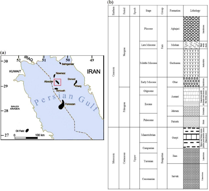
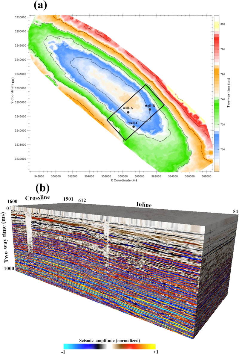
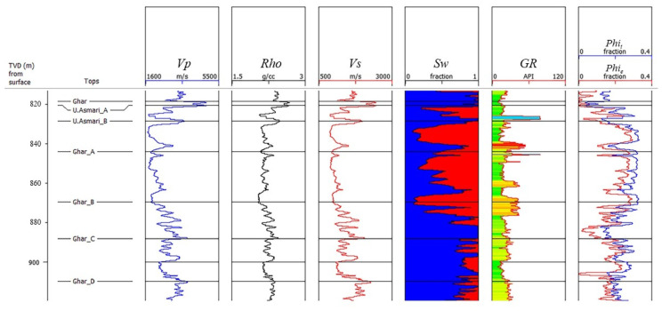
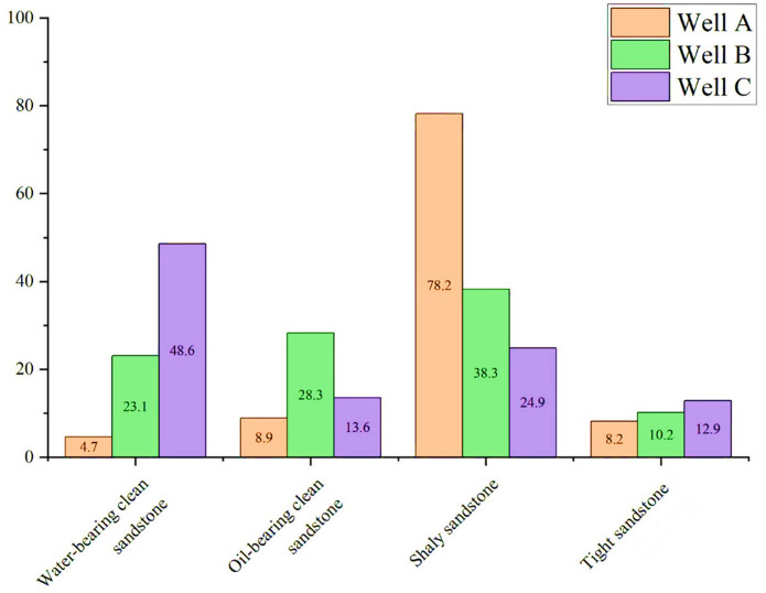
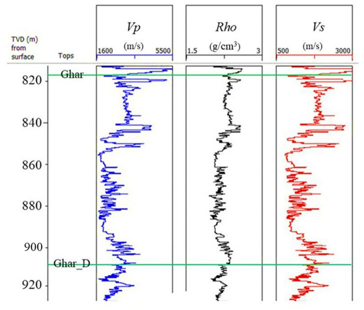
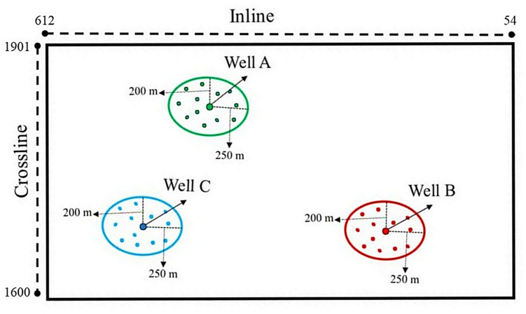
This study presents a hybrid seismic inversion framework to estimate 3D acoustic impedance volumes in a geologically complex and data-limited environment. The approach integrates physics-informed pseudo-well generation, based on calibrated rock physics modeling and variogram statistics, with a deep feedforward neural network (DFNN) that maps multi-attribute seismic data to acoustic impedance while substantially reducing dependence on low-frequency background models and dense well calibration. The compact DFNN serves as a high-dimensional nonlinear mapper that learns the relationship between seismic attributes and impedance logs, a task for which it is well suited, leading to accurate predictions. We generated synthetic elastic logs (compressional and shear velocities, and bulk density) using calibrated rock physics modeling and variogram-constrained stochastic simulation to supplement real well logs. We produced a lithologically diverse and statistically coherent training dataset. This process, applied to only 3 real wells, generated a robust ensemble of 36 synthetic pseudo-wells, effectively addressing the severe data scarcity and providing sufficient training data. Seismic attributes representing amplitude, phase, and frequency characteristics are selected to facilitate the model's ability to resolve subtle geological heterogeneity. The trained DFNN is validated through a leave-one-well-out strategy yielding a cross-correlation coefficient of up to 95.4% and a normalized relative error below 1% when tested on the blind wells. Combining physical modeling with data-driven learning reduces reliance on low-frequency background models and dense calibration. Rather than replacing conventional inversion, it provides a complementary, geologically consistent, and computationally efficient approach for reliable reservoir characterization in offshore environments. Future work may focus on incorporate uncertainty quantification and volumetric convolutional networks to further improve spatial resolution and model reliability in complex subsurface settings.

Keywords: Acoustic impedance; DFNN; Pseudo-well generation; Rock physics modeling; Seismic inversion.

Fig. 1

(a) Regional base map of the Persian Gulf region, delineating the Aboozar oilfield study area (indicated by the red square), and (b) stratigraphic column showing the major formations in this oilfield.

Fig. 2

(a) The contour map derived from 3D seismic data of the Ghar Formation in Aboozar oilfield with well locations. (b) The 3D seismic data of the Aboozar oilfield.

Fig. 3

Petrophysical logs (V_P, Rho, V_S, Sw​, GR, Phi_T/Phi_e) of Well A within the Ghar–Ghar D interval.

Fig. 4

A flowchart for predicting a 3D acoustic impedance volume trained by a neural network on pre-stack seismic data and petrophysical logs.

Fig. 5

Rock physics modeling of Well A (logs of V_P, V_S, and density with their corresponding predictions).

Fig. 6

Cross plots of (a) V_P vs. V_S, (b) V_P vs. MSI, (c) V_p vs. Rho, and (d) V_p vs. Phi_e in Well A.

Fig. 7

Quantitative QC plots for predicted values ​​of (a) V_p, (b) V_S, and (c) Rho of Well A (PQ, CC, and NRMSE are determined for each value which quantitatively shows that the RPM has high accuracy).

Fig. 8

Lithofacies distribution (Ghar to Ghar D Interval). Proportional representations show four lithofacies (oil-bearing clean sandstone, water-bearing clean sandstone, silty shale, tight sandstone) classified by shale volume (shale), Phi_e, and Sw in wells (a) A, (b) B, and (c) C.

Fig. 9

Comparison of the distribution of rock facies in wells A, B, and C in the Ghar to Ghar D interval. The stacked bar graph shows the percentage of four lithofacies classified by shale volume (shale), Phi_e, and Sw.

Fig. 10

Distribution of the four defined lithofacies (oil-bearing clean sandstone, water-bearing clean sandstone, silty shale, tight sandstone) with measured depth across the Ghar to Ghar D interval in wells A, B, and C.

Fig. 11

Fundamental and initial stages of the sequential workflow for constructing a pseudo-well for well A across the Ghar to Ghar D interval (measured depth: 818.5–909.4 m). (a) Calibration curves derived from RPM for both observed (blue) and predicted (orange) values of V_P (left) and Rho (right); (b) comparison of elastic properties (blue) with their corresponding trends (orange) for V_P (left) and Rho (right); (c) comparison between observed (blue) and background (orange) trends for Phi_T (left) and MSI (right); and (d) residual analysis of Phi_T (left) and MSI (right) relative to their background trends.

Fig. 12

Final stages of the sequential workflow for constructing a pseudo-well for Well A across the Ghar to Ghar D interval (measured depth: 818.5–909.4 m). (a) Vertical variogram modeling of Phi_T residuals using a Gaussian model; and (b) multi-property quality control by generating ten Gaussian realizations to evaluate the accuracy of the model in reproducing the variability observed within the original log data (Phi_T, V_S, V_P, and Rho).

Fig. 13

Logs of V_P, V_S, and Rho for a representative pseudo-well generated around real Well A. This pseudo-well is located within a statistically valid elliptical neighborhood offset from the real well, based on the spatial constraints defined by the variogram model. The logs span the Ghar to Ghar-D interval and exhibit realistic elastic trends consistent with the lithological framework of the field.

Fig. 14

Spatial layout of 36 pseudo-wells generated around real wells A, B, and C within elliptical neighborhoods defined by variogram-informed lateral offsets (± 250 m inline, ± 200 m crossline). The layout ensures statistical independence and full seismic coverage. While the surface locations are shown for clarity, they are illustrative only; the pseudo-wells serve as statistically and petrophysically valid training samples, and exact placement is not critical.

Fig. 15

Predicted 3D acoustic impedance volume generated by a DFNN, trained using seismic attributes and augmented well data. The output cube covers the range of Inline 54–612, Crossline 1600–1900, and TWT from 730 to 790 ms, and encompasses the interval of interest from Ghar to Ghar-D. The model, leveraging both real and pseudo-well logs, demonstrates spatially consistent impedance variations that reflect the geological structure across the seismic volume.

Fig. 16

Scatter plot of predicted vs. actual P-impedance (with 1:1 reference line) based on 948 samples from 39 wells—3 real wells and 36 synthetic pseudo-wells. Markers are coded by data origin: real wells (A, B, C) are listed explicitly in the legend, while pseudo-wells follow the labels Pseudo.W.[A/B/C] _01_sim_XXXX (12 per real well; 36 total). Pseudo-wells were used for training/augmentation only; reported validation statistics are computed on real wells. Predictions were obtained with a DFNN (three hidden layers of nine nodes each) trained on seven seismic attributes, yielding a cross-correlation of 95.4% and an RMSE of 0.592.

Fig. 17

(a) Normalized seismic amplitude section (pre-inversion) along inline 148 to 610 at crossline 1600, highlighting the study interval from Ghar to Ghar_D. (b) Corresponding P-wave acoustic impedance volume (post-inversion) predicted by the trained DFNN. Compared to the raw seismic data, the inversion output exhibits enhanced stratigraphic resolution, improved vertical continuity, and clearer delineation of subsurface heterogeneities. The main low-impedance anomaly within the target interval is clearly indicated, corresponding to the interval of interest.

References

1. Zhao, L., Nasser, M. & h. Han, D. Quantitative geophysical pore-type characterization and its geological implication in carbonate reservoirs. Geophys. Prospect.61, 827–841. 10.1111/1365-2478.12043 (2013).
1. Dvorkin, J., Gutierrez, M. A. & Grana, D. Seismic Reflections of Rock Properties (Cambridge University Press, 2014). 10.1017/CBO9780511843655
1. Russell, B. H., Hedlin, K. J. & N1-N14. Extended poroelastic impedance. Geophysics84. 10.1190/geo2018-0311.1 (2019).
1. El-Sayed, A. S., Mabrouk, W. M. & Metwally, A. M. Pre-stack seismic inversion for reservoir characterization in pleistocene to pliocene channels, Baltim gas field, Nile Delta, Egypt. Sci. Rep.15, 1180. 10.1038/s41598-024-75015-x (2024). - PMC - PubMed
1. Moseley, B., Markham, A. & Nissen-Meyer, T. Fast approximate simulation of seismic waves with deep learning. ArXiv Preprint arXiv:1807 06873. 10.48550/arXiv.1807.06873 (2018).
LinkOut - more resources