Mathematical linearity of circulatory transport

Abstract

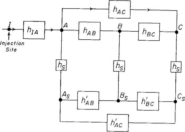
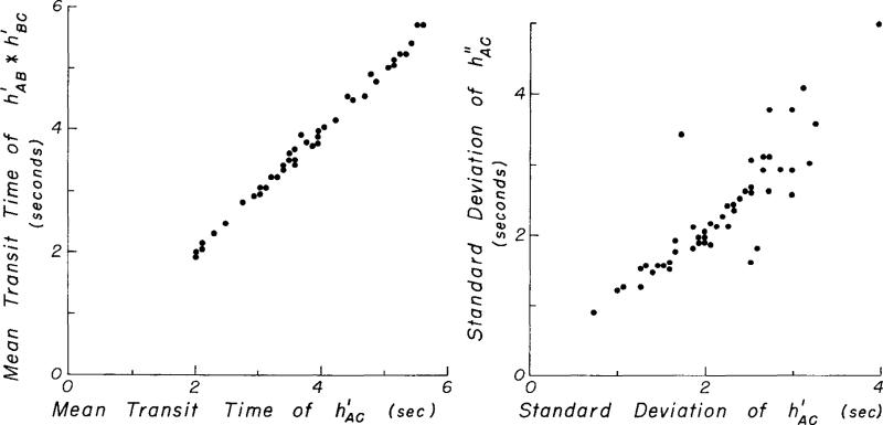
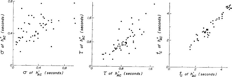
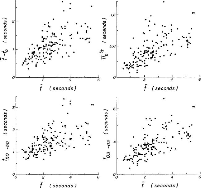
After injections of indocyanine green into the pulmonary artery or left ventricle of anesthetized dogs, indicator-dilution curves were recorded, via identical short sampling systems, from the root of the aorta, the lower thoracic aorta, and the bifurcation of the aorta. The distributions of transit times (transport functions) between each of the three pairs of sampling sites were determined in terms of a mathematical model using the whole of each recorded curve. The accuracy of each transport function was demonstrated by convoluting it with the upstream dilution curve to produce a theoretical downstream dilution curve closely matching the recorded downstream dilution curve. Linearity and stationarity of the aortic system were then tested by comparing the convolution of the transport functions of the upper and lower segments of the aorta with the transport function from aortic root to bifurcation. The results indicate that it is reasonable to apply the superposition principle, as is assumed when calculating flows or mean transit times by indicator-dilution methods, and that cardiac fluctuations in flow produce relatively little error.

FIG. 1

Block diagram of the experiment. The bolus of injectate introduced at I (pulmonary artery or left ventricle) is somewhat dispersed in the vascular system by the process h_IA(t) before it reaches the three aortic sampling sites A, B, and C. The sampling system transport functions, h_s(t), were identical, so that the transport functions $h_{\mathrm{AB}}^{\prime }\left(t\right)$, $h_{\mathrm{BC}}^{\prime }\left(t\right)$, or $h_{\mathrm{AC}}^{\prime }\left(t\right)$ between pairs of the simultaneously recorded curves A_s, B , and C_s, would be the same as the transport functions h_AB, h_BC, or h_AC between the corresponding pairs of the actual arterial curves.

FIG. 2

Aortic transport functions. Left panels: recorded curves A_s, B_s, and C_s are shown by the continuous lines. ${\mathrm{B}}_s^{\prime }={\mathrm{A}}_s{}^{\ast }{h}_{\mathrm{AB}}^{\prime }$ (triangles) (the asterisk denotes the process of convolution); ${\mathrm{C}}_s^{\prime }={\mathrm{B}}_s{}^{\ast }{h}_{\mathrm{BC}}^{\prime }$ (circles); and ${\mathrm{C}}_s^{″}={\mathrm{A}}_s{}^{\ast }{h}_{\mathrm{AC}}^{\prime }$ (plus signs). Right panels: convolution of the transport functions h_AB and h_BC should be the same as h_AC if the whole system is linear. The test is only as good as the weakest of the representations of h_AB by $h_{\mathrm{AB}}^{\prime }$, of h_BC by $h_{\mathrm{BC}}^{\prime }$, and of h_AC by $h_{\mathrm{AC}}^{\prime }$. However, the result that $h_{\mathrm{AB}}^{\prime }{}^{\ast }{h}_{\mathrm{BC}}^{\prime }=h_{\mathrm{AC}}^{″}\left(t\right)$ (plus signs) is similar to $h_{\mathrm{AC}}^{\prime }\left(t\right)$ is strong evidence that the system is linear and stationary.

FIG. 3

Aortic transport functions (double injection into pulmonary artery). The convolution of the estimated transport functions, $h_{\mathrm{AB}}^{\prime }{}^{\ast }{h}_{\mathrm{BC}}^{\prime }$, results in a theoretical curve, $h_{\mathrm{AC}}^{″}\left(t\right)$ (plus signs, right panel) which is similar to the experimental estimate of the transport function $h_{\mathrm{AC}}^{\prime }$ between the aortic arch and the bifurcation of the aorta.

FIG. 4

Comparison of mean transit time and standard deviation of theoretical and observed aortic transport functions. The equation for the data in the left panel is ${\stackrel{‒}{t}}_{h\mathrm{AC}}^{″}=0.032+0.998{\stackrel{‒}{t}}_{h_{\mathrm{AC}}}^{\prime }$ (N = 54, r = 0.997) and for the right panel is $\pi {2^{1∕2}}_{h_{\mathrm{AC}}^{″}}=0.139+1.18\pi {2^{1∕2}}_{h_{\mathrm{AC}}^{\prime }}$ (N = 54, r = 0.87), in which π2 is the variance and π2^1/2 is the standard deviation. (One dot represents more than one data point on these plots when the points coincide.)

FIG. 5

Comparison of the parameters of $h_{\mathrm{AC}}^{″}$ with those of $h_{\mathrm{AC}}^{\prime }$. Regression equations for 54 sets are σ_h″ = 0.25 + 0.58 σ_h′ (sd = 0.16); τ_h″ = –0.24 + 1.26 τ_h′ (sd = 0.21); and t_ch″ = –0.07 + 1.02 t_ch″ (sd = 0.21).

FIG. 6

Comparison of convolution of upstream curve with theoretical and observed transport functions. The curves are those shown in Figs. 2 (lower) and 3. The upstream curve A_s was convoluted with both the theoretical ($h_{\mathrm{AC}}^{″}\left(t\right)$) and observed ($h_{\mathrm{AC}}^{\prime }\left(t\right)$) transport functions, resulting in two theoretical downstream curves (the X's and O's, respectively) which can be compared with the recorded downstream curve, C_s.

FIG. 7

Parameters of spread of transport function. Various parameters of an average aortic transport function are shown. t_03–03 may be considered the passage time of the curve although it is slightly shorter than the maximal measurable passage time.

FIG. 8

Effect of mean transit time on temporal dispersion of indicator in canine aorta.

References

1. Bassingthwaighte JB. Plasma indicator dispersion in arteries of the human leg. Circulations Res. 1966;19:332–346. - PMC - PubMed
1. Bassingthwaighte JB, Ackerman FH, Wood EH. Applications of the lagged normal density curve as a model for arterial dilution curves. Circulation Res. 1966;18:398–415. - PMC - PubMed
1. Bassingthwaighte JB, Anderson D, Knopp TJ. Effects of unsteady flow on indicator dilution in the circulation. Proc. Ann. Conf. Engnr. Med. Biol., 8th. 1966:184.
1. Bassingthwaighte JB, Edwards AWT, Wood EH. Areas of dye-dilution curves sampled simultaneously from central and peripheral sites. J. Appl. Physiol. 1962;17:91–98. - PubMed
1. Bassingthwaighte JB, Edwards AWT, Wood EH. Use of an optical density ruler in measurements of dye-dilution curves. J. Appl. Physiol. 1964;19:347–353. - PMC - PubMed
LinkOut - more resources