

doi: 10.1016/0025-5564(94)90037-x.
A G protein-based model of adaptation in Dictyostelium discoideum
Affiliations
- PMID: 8155908
- PMCID: PMC6388623
- DOI: 10.1016/0025-5564(94)90037-x
Item in Clipboard
A G protein-based model of adaptation in Dictyostelium discoideum
Math Biosci.
1994 Mar.
Abstract
A new model is proposed based on signal transduction via G proteins for adaptation of the signal relay process in the cellular slime mold Dictyostelium discoideum. The kinetic constants involved in the model are estimated from Dictyostelium discoideum and other systems. A qualitative analysis of the model shows how adaptation arises, and numerical computations show that the model agrees with observations in both perfusion and suspension experiments. Several experiments that can serve to test the model are suggested.
Figures
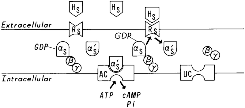
A schematic diagram of the activation of adenylate cyclase via Gs proteins. Hs denotes the stimulus signal, Rs the stimulus receptor, αsGDPβγ unactivated Gs protein, and UC unactivated adenylate cyclase. It is believed that upon binding of Hs with Rs, Gs is activated by the HsRs complex. This involves the release of the βγ subunits and the addition of GTP to the αs chain. αsGTP, which is denoted by in this figure, then activates adenylate cyclase, which catalyzes the conversion of ATP to cAMP.
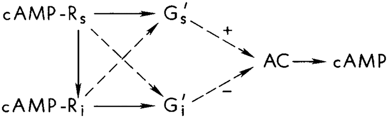
The scheme of interactions for the regulation of AC proposed by van Haastert and coworkers [–41].
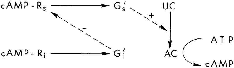
A schematic diagram of the interactions in the proposed model. An extracellular cAMP stimulus serves as both the stimulus and the inhibitory signal. Adaptation arises from the action of on the hormone–receptor cmplex. Viewed at the level of cAMP production, this interaction produces a feedforward mechanism for the control of cAMP production.
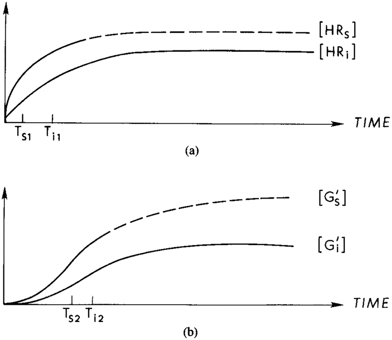
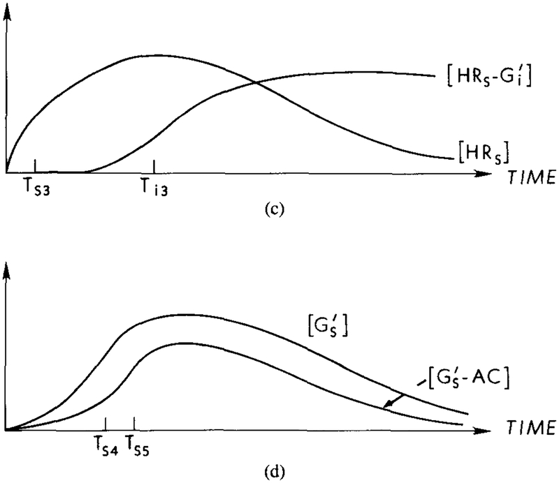
A qualitative description of latency and adaptation in the signal transduction process under a constant stimulus. The time for activation of G protein is the major component of the latency between stimulus arrival and activation of the adenylate cyclase. Adaptation at the receptor level results from the interaction of with HRs, which reduces the amount of activated Gs and cyclase. (a) Response curves for HRs and HRi under a constant stimulus. Ts1 and Ti1, represent the half-maximal times for the respective components. The dashed line indicates the response for HRs in the absence of an inhibitory effect. (b) Response curves for the concentrations of and . Ts2 and Ti2 represent the half-maximal times for the respective components. The dashed line indicates the response if the inhibitory effect is not present. (c) In the presence of , HRs is diminished due to the formation of . The half-maximal time, Ts3, for HRs in the presence of is approximately the same as Ts1, whereas Ti3 > Ti2. (d) Response curves for the concentration of and . The half-maximal time for , Ts4, is approximately equal to Ts2, whereas the half-maximal time for , Ts5, is greater than Ts4. The rate of cAMPi production is proportional to the concentration of GsAC.
A qualitative description of latency and adaptation in the signal transduction process under a constant stimulus. The time for activation of G protein is the major component of the latency between stimulus arrival and activation of the adenylate cyclase. Adaptation at the receptor level results from the interaction of with HRs, which reduces the amount of activated Gs and cyclase. (a) Response curves for HRs and HRi under a constant stimulus. Ts1 and Ti1, represent the half-maximal times for the respective components. The dashed line indicates the response for HRs in the absence of an inhibitory effect. (b) Response curves for the concentrations of and . Ts2 and Ti2 represent the half-maximal times for the respective components. The dashed line indicates the response if the inhibitory effect is not present. (c) In the presence of , HRs is diminished due to the formation of . The half-maximal time, Ts3, for HRs in the presence of is approximately the same as Ts1, whereas Ti3 > Ti2. (d) Response curves for the concentration of and . The half-maximal time for , Ts4, is approximately equal to Ts2, whereas the half-maximal time for , Ts5, is greater than Ts4. The rate of cAMPi production is proportional to the concentration of GsAC.
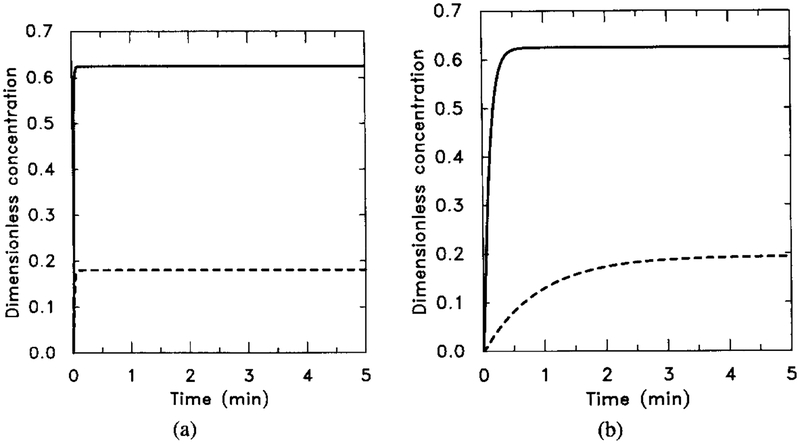
The response of the uncoupled system. The stimulus is [H] = 0.1 μM for t ∈ (0, 5). The numerical results can be compared with the analytical results obtained from the analysis in Section 4 and with Figure 6 to verify the steady-state additivity of the uncoupled system. (a) The dimensionless concentrations of HRs (solid line) and HRi (dashed line). (b) The dimensionless concentrations of (solid line) and (dashed line). Note that the half-time for the buildup of agrees well with the theoretical estimate but that the rise time for is longer than the theoretical estimate. This discrepancy indicates that the pseudo-steady-state hypothesis applied to [HRsGs] is probably not valid on this time scale.
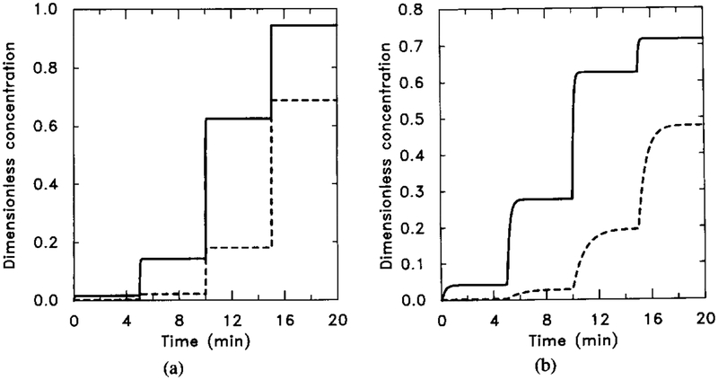
The response of the uncoupled system to sequential increases of the stimulus. The sequence is [H] = 0.001 μM for t ∈ (0, 5); [H] = 0.001 μM for t ∈ (5, 10); [H] = 0.1 μM for t ∈ (10, 15); and [H] = 1.0 μM for t ∈ (15, 20). (a) The dimensionless concentrations of HRs (solid line) and HRi (dashed line). (b) The dimensionless concentrations of (solid line) and (dahsed line).
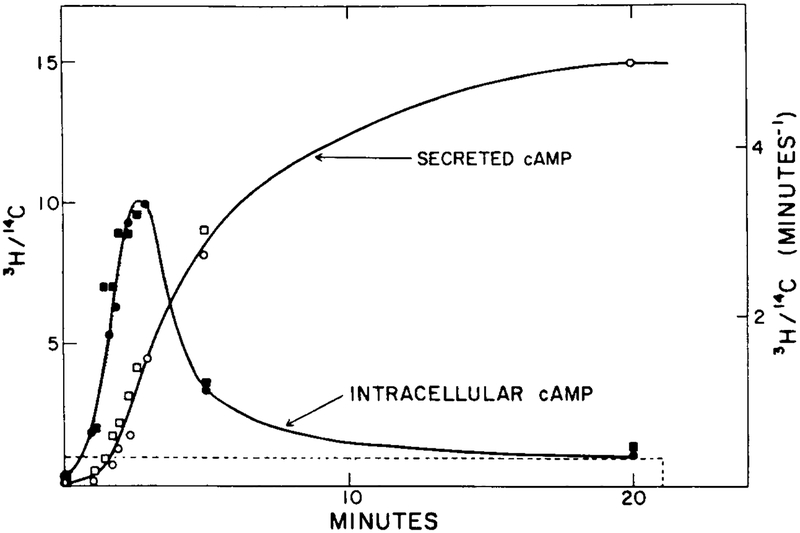
The experimental response of cAMP secretion to a single prolonged stimulus of 10−6 M extracellular cAMP (from [11]). The stimulus is a 20-min step function of 1 μM magnitude (dashed line). Two experimental results (circles and squares) are shown here for intracellular cAMP concentration (filled symbols) and cAMP secretion (open symbols).
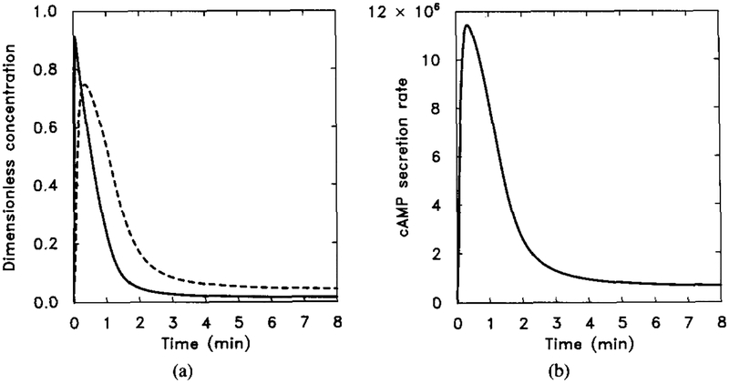
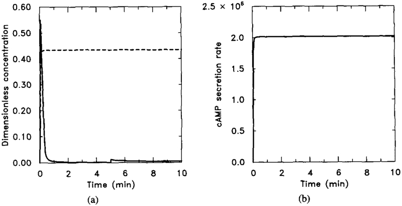
The response of the model to a prolonged stimulus of 10−6 M extracellular cAMP. The stimulus is [H] = 1.0 μM from t = 0 to t = 8 min. (a) The dimensionless concentrations of HRs (solid line) and cAMPi/10 (dashed line). (b) The dimensional secretion rate of cAMPi in molecules per cell per minute. Compare with Figure 7 for experimental data.
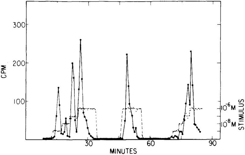
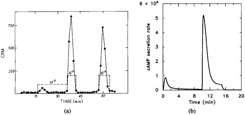
The experimentally observed cAMP secretion in response to a multistep stimulus. The first step is from 0 to 10−9 M, and this is followed by three 10-fold increases. (Adapted from [9].)
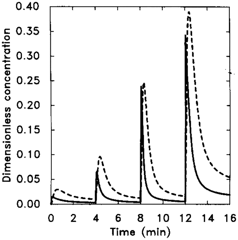
The numerical response of the system using the measured k−1. Starting at t = 0 min, extracellular cAMP was increased from 0 to 10−9 M and then to 10−6 M in three 10-fold steps of 4 min duration. Dimensional parameter values are given in Table 4. The dimensionless concentrations of HRs (solid line) and cAMPi/10 (dashed line).
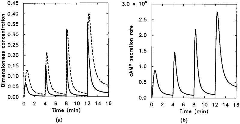
The numerical response to sequential 10-fold increases of stimuli with k−1 in Table 4 changed from 0.45 to 0.075. Other parameter values are unchanged. The stimulus is the same as in Figure 10. (a) The dimensionless concentrations of HRs (solid line) and cAMPi/10 (dashed line). (b) The dimensional secretion rate of cAMPi (molecules per cell per minute). Compare with Figure 9 for experimental data.
The experimental and model response to a two-step sequential stimulus. Note that after removal of the stimulus the unadapted portion decays very rapidly. The parameter value are the same as in Figure 11. The stimulus sequence is [H] = 10−9 M for t = 0 to t = 10, [H] = 10−6 M for t = 10 to t = 15, and [H] = 0 M for t = 15 to t = 20. (a) The experimentally observed response (adapted from [9]). (b) The dimensional secretion rate of cAMPi in molecules per cell per minute.
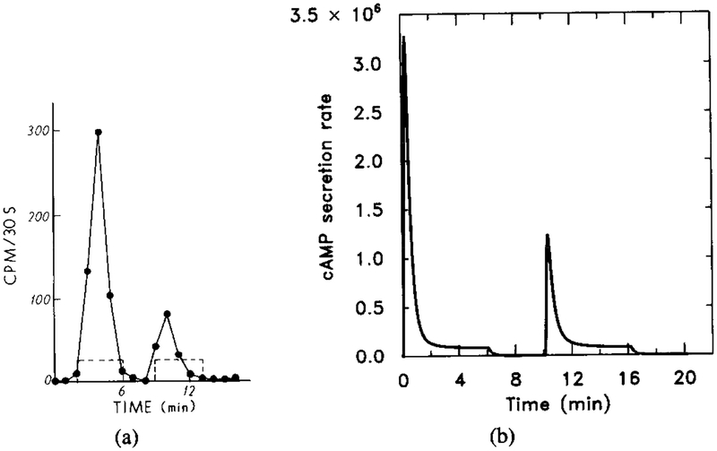
The experimental and numerical response to short two-step stimuli. The time course of the extracellular cAMP stimulus is 10−8 M (t = 0–6), 0 M (t = 6–10), 10−8 M (t = 10–16), and 0 M (t = 16–20). This experiment probes the time course of deadaptation, because the magnitude of the response to the second stimulus depends upon the degree to which the cells have recovered from the first stimulus. Parameter values are the same in Figure 11. (a) Experimental results (adapted from [11]). (b) The dimensional secretion rate of cAMPi (molecules per cell per minute). The response to the second signal of the same magnitude is much smaller because has not decayed completely. The magnitude of the second response increases with the elapsed time since the preceding signal.
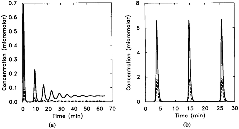
The dimensionless [cAMPi] as a function of time, illustrating decaying oscillations. Parameter values are taken from Tables 8 and 13. The initial stimulus is [H] = 10−8 M. In this figure we scale both γ2 and γ5 by a factor f. Here γ2 = f × 0.048, and γ5 = f × 0.224, with f = 5.0. (b) A stable oscillation for f = 10.0. Shown are the dimensional intracellular cAMP concentration [cAMPi] (solid line) and 10 times the extracellular cAMP concentration [cAMPo] (dashed line).
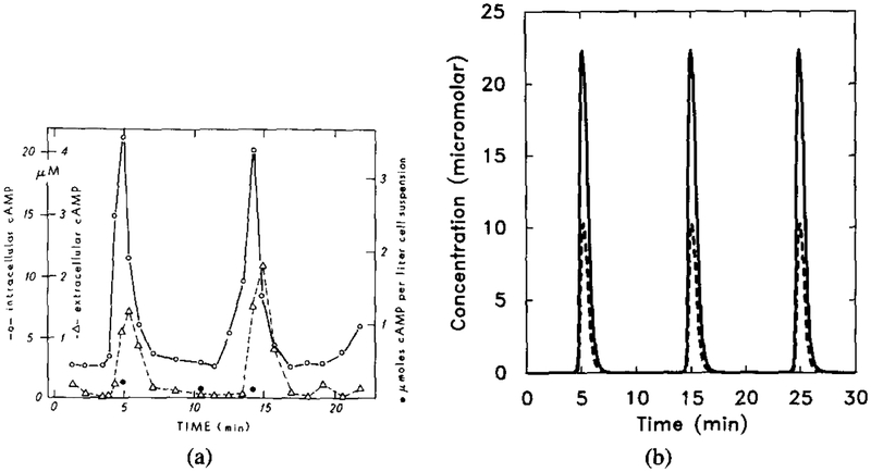
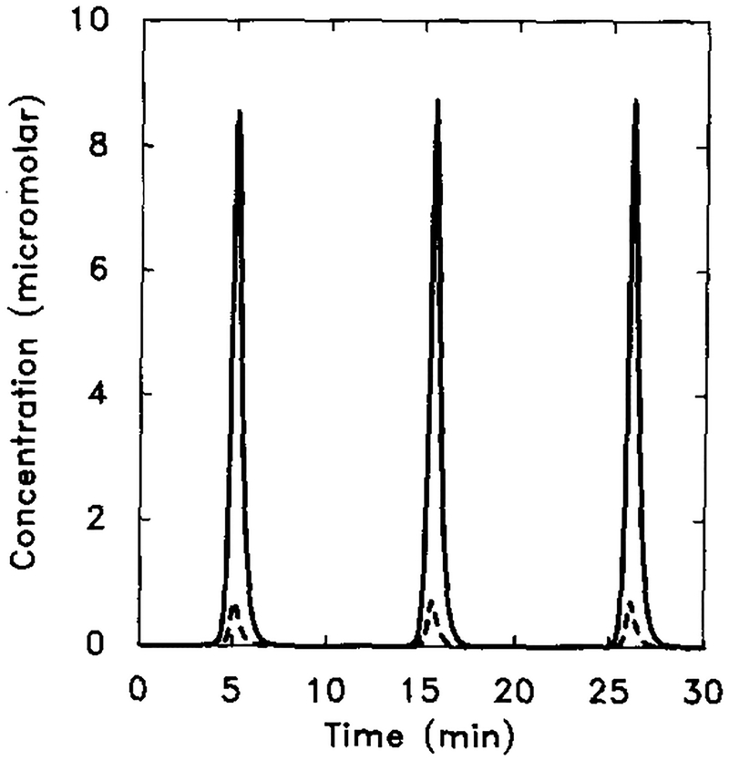
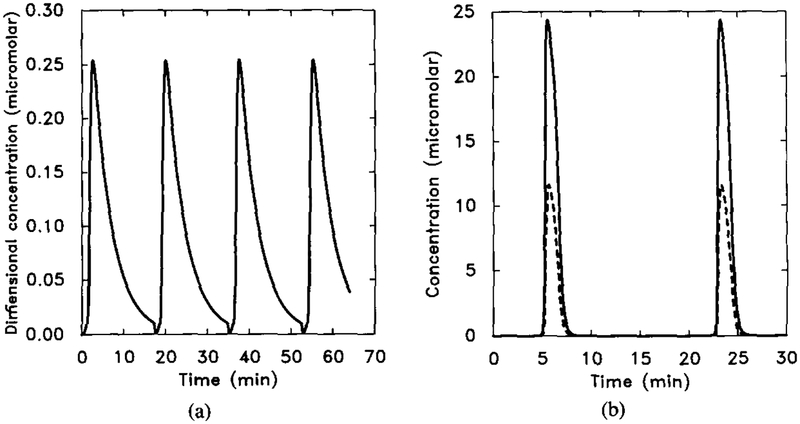
The experimental results for oscillations in suspensions and the corresponding numerical results. Parameter values are the same as in Figure 14 except f = 25.0. (a) Experimental measurements of intracellular (◯) and extracellular (Δ). Redrawn from Figure 2 of Gerisch and Wick [20]. (b) Dimensional intracellular cAMP concentration [cAMPi] (solid line) and five times the extracellular cAMP concentration [cAMPo] (dashed line).
The magnitude of oscillation is significantly influenced by the parameters reflecting the activities of AC, iPDE, and mPDE. Here γ6 is decreased by a factor of 10 (γ6 = 0.29) and other parameter values are the same as in Figure 15. Shown are the dimensional intracellular cAMP concentration [cAMPi] (solid line) and 10 times the extracellular cAMP concentration [cAMPo] (dashed line).
An illustration of how changes in β2 and β5 significantly change the oscillation frequency. Here β2 and β5 are divided by a factor of 2. Other parameter values are the same as in Figure 15. Compare with Figure 15. (a) The dimensionless concentration of . (b) Five times the intracellular cAMP concentration [cAMPi] (solid line) and the extracellular cAMP concentration [cAMPo] (dashed line).
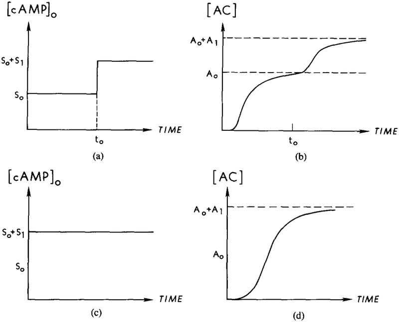
The steady-state additivity of cAMP production in the response to an extracellular cAMP signal, predicted for cholera toxin–treated cells. The steady-state concentration should depend only on the final stage of extracellular stimulus and not on the stimulus history. (a) A two-step stimulus of magnitude from S0 to S0 + S1. (b) The corresponding response of activated adenylate cyclase to the stimulus in (a). The steady-state concentration should be from A0 to A0 + A1. (c) A single-step stimulus of magnitude S0 + S1. (d) The corresponding response of activated adenylate cyclase to the stimulus in (c).
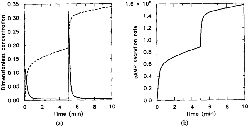
The effect of cholera toxin as predicted by the model. The result should be compared with Figure 18 to see the steady-state additivity. Parameter values are given in Table 4 with k5 = 0 to mimic the effect of cholera toxin. The stimulus is 10−8 M for t ∈ (0, 5) and 10−7 M for t ∈ (5, 10). (a) Dimensionless concentrations of HRs (solid line) and cAMPi/10 (dashed line). (b) Dimensional secretion rate of cAMPi (molecules per cell per minute).
Numerical output for the experiment when GTP is replaced by GTPγS. The parameter values are the same as in Figure 19 with h5 = 0 to simulate the fact that αi-GTPγS is also nonhydrolyzable. The stimulus is 10−8 M for t ∈ (0, 5) and 10−7 M for t ∈ (5, 10). (a) Dimensionless concentrations of HRs (solid line) and cAMPi/10 (dashed line). (b) Dimensional secretion rate of cAMPi (molecules per cell per minute). (b) should be compared with (b) in Figure 19.
References
-
- Adawia A, Jasper JR, I’. A Insel, and H. J. Motulsky, Stoichiometry of receptor-Gs-adenylate cyclase interactions, FASEB J 52300–2303 (1991). - PubMed
-
- Asano T, Katada T, Gilman A, and Ross E, Activation of the inhibitory GTP-binding protein of adenylate cyclase, Gi, by β-adrenergic receptors in reconstituted phospholipid vesicles, J. Biol. Chem 259(1.5):9351–9354 (1984). - PubMed
-
- Berridge M, Inositol trisphophate and diacylglycerol: two interacting second messengers, Ann. Rev. Biochem 56:159–193 (1987). - PubMed
-
- Bominaar A, Snaar-Jagalska B, Kesbeke F, and van Haastert P, Signal-transducing G proteins in Dictyosteliun discoideum, in the guanine nucleotide binding proteins Common structural and functional properties (NATO ASI, Vol. 165) Bosch L, et al. eds., Springer-Verlag, Berlin, 1989, pp. 369–375.
Publication types
MeSH terms
Substances
Grants and funding
LinkOut - more resources
Full Text Sources
