Use of radial density plots to calibrate image magnification for frozen-hydrated specimens

Abstract

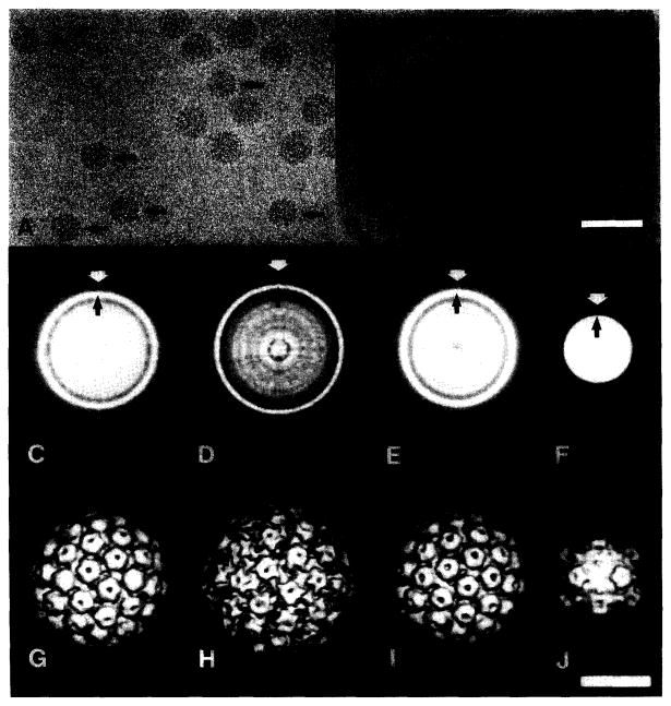
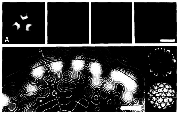
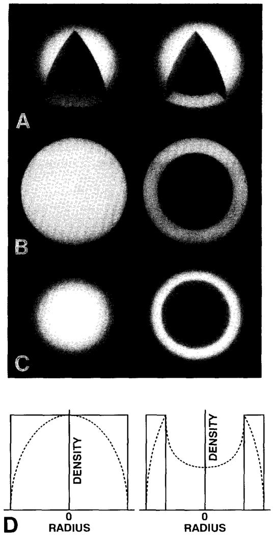
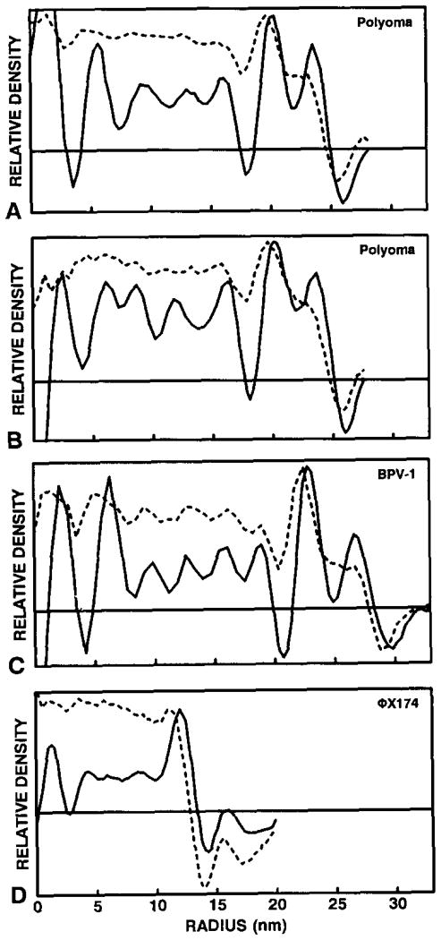
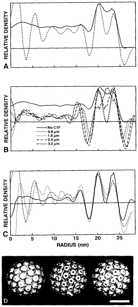
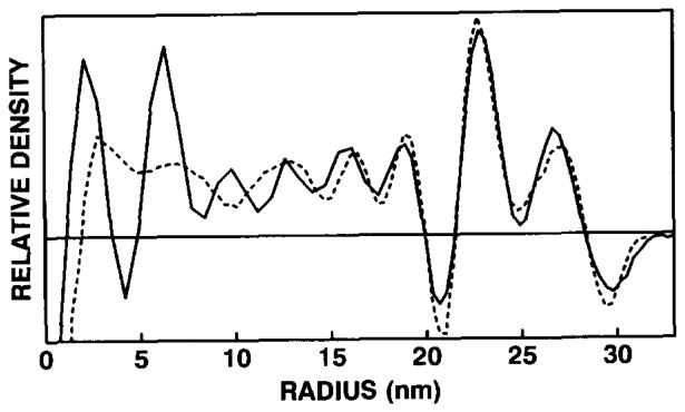
Accurate magnification calibration for transmission electron microscopy is best achieved with the use of appropriate standards and an objective calibration technique. We have developed a reliable method for calibrating the magnification of images from frozen-hydrated specimens. Invariant features in radial density plots of a standard are compared with the corresponding features in a "defocused" X-ray model of the same standard. Defocused X-ray models were generated to mimic the conditions of cryo-electron microscopy. The technique is demonstrated with polyoma virus, which was used as an internal standard to calibrate micrographs of bovine papilloma virus type 1 and bacteriophage phi X174. Calibrations of the micrographs were estimated to be accurate to 0.35%-0.5%. Accurate scaling of a three-dimensional structure allows additional calibrations to be made with radial density plots computed from two- or three-dimensional data.

Fig. 1

Use of polyoma virus as an internal standard in unstained, frozen-hydrated preparations: (A) Mixture of polyoma and BPV-1. Polyoma (arrows) is distinguished from BPV-1 by its slightly smaller size. (B) Mixture of polyoma and ΦX174. Several empty ΦX174 particles are also present. Apical caps on the ΦX174 particles may be observed as faint projections on the capsid periphery. (C–F) CAD images (in reverse contrast) of polyoma (C) and BPV- 1 (D) from image (A), and polyoma (E) and ΦX174 (F) from image (B). CAD images were computed from averages of 43 (C), 10 (D), 12 (E), and 57 (F) particle images. White arrows identify approximate particle edges used to calibrate magnification according to the method of Olson and Baker [5]. The bright rings (black arrows) correspond to the highest density peaks near the inner radius of the capsid shell. The CAD image of ΦX174 (F) is distinct from the papovavirus CAD images (C–E) because the apical caps, the density feature at maximum diameter (white arrow), gives rise to a faint ring. The average radius of the shell's inner wall (black arrow) is the most prominent CAD feature at higher radii. (G–J) Surface-shaded views (along icosahedral two-fold axes) of polyoma (G) and BPV-1 (H) computed from 21 and 6 particle images, respectively (from (A)), and polyoma (I) and ΦX174 [28] (J) computed from 11 and 25 particle images, respectively (from (B)). Bar = 100 nm (A, B) and 25 nm (C–J).

Fig. 2

Measurements of particle diameters from the three-dimensional reconstruction of polyoma shown in fig. 1G. This illustrates the difficulties encountered in defining the particle–solvent boundary. (A) Planar sections through the reconstruction, perpendicular to an icosahedral three-fold axis of symmetry. (This is where interparticle contacts were found in crystals used for X-ray diffraction experiments [17].) The centers of the four sections are at radii of 23.9, 24.6, 25.3 and 26.0 nm (left to right). The choice of which section contains protein density at highest radius depended on how the data were displayed (e.g. positive versus negative contrast, color versus black-and-white, and contrast-enhanced look-up tables). (B) Contoured, grey-level display of an equatorial section (left) from the reconstruction. The section passes through the axes of adjacent pentavalent (arrow identifies the icosahedral five-fold axis) and hexavalent capsomeres. The arc is drawn at a radius of 24.8 nm and corresponds to the interparticle packing distance determined by X-ray crystallography [17]. Low-magnification views of the reconstruction are shown in a central section (far right, top; in the same orientation as left) and surface-shaded representation (far right, bottom; particle rotated 90° about a horizontal axis). The line in the shaded view indicates the plane of the equatorial sections. Bar = 25 nm (A) and 5 nm (B).

Fig. 3

Solid sphere (left) and spherical shell (right) models of uniform density used to illustrate the properties of CAD and SAD plots. (A) Surface-shaded views cut open to reveal solid core of sphere and empty core of shell. (B) Equatorial sections of (A). (C) Projected images of (A). (D) SAD (———) and CAD (- - - - - -) plots of (A) and (C), respectively. Peak values in the corresponding CAD and SAD plots were normalized, which artificially reduces the absolute scale of the CAD plot relative to the SAD plot.

Fig. 4

Comparisons of calibrated CAD (- - - - - -) and SAD (———) plots of polyoma from BPV-1 (A) and ΦX174 (B) micrographs, and BPV-1 (C) and ΦX174 [28] (D). The highest peak values of each CAD/SAD pair in the region ~ 18–26 nm for polyoma, ~ 21–30 nm for BPV-1, and ~ 10–14 nm for ΦX174 were normalized. Note the differences between SAD and CAD, especially in the capsid region (compare to fig. 3). Large fluctuations in the SAD plots near the origin are artifacts generated by the Fourier Bessel procedures used to compute the three-dimensional reconstructions. The horizontal line in each graph represents the zero density level.

Fig. 5

Comparison of polyoma EM and X-ray data. (A) SAD plots computed from “native” X-ray model (———) and EM reconstruction (- - - - - - -) (from the BPV-1 micrograph, fig. 1A) data, showing marked differences in the two types of data. The highest peak values in the capsid region (r = 18−26 nm) were normalized. (B) SAD plots of the X-ray model at various underfocus levels: native (———) (no CTF applied). 0.8 μm (- - - - - -), 1.6 μm (· · · · · ·), 2.4 μm (– – –), and 3.2 μm (–··–··–), showing the effects of treating the X-ray data with theoretical CTFs. The highest peak values in the capsid region were normalized. (C) SAD calibrations of two polyoma reconstructions ((- - - - - -) from the BPV-1 micrograph, and (· · · · · ·) from the ΦX174 micrograph) with the 1.6 μm underfocused X-ray model (———). Calibrations were made by comparing densities in the capsid region from r = 18−26nm. (D) Surface-shaded views (along two-fold axes of symmetry and contoured at comparable density thresholds) of the “native” (left) and 1.6 μm underfocused (middle) X-ray models, and the polyoma reconstruction (right) obtained from the ΦX174 micrograph. Bar = 25 nm. The “defocused” X-ray map resembles the reconstructed EM map more closely in appearance and SAD than does the unaltered structure. The horizontal line in each graph represents the zero density level.

Fig. 6

SAD plots showing the calibration of a 77-particle, BPV-1 reconstruction [23] (- - - - - -) with the 6-particle BPV-1 reconstruction (———). The two plots were calibrated for density values at radii between 21.4 and 28.4 nm. The poor correlation of densities at r < 19 nm, corresponding to the nucleohistone core, is consistent with the notion that the core components are not organized with icosahedral symmetry [21]. The horizontal line represents the zero density level.

References

1. Backus RC, Williams RC. J Appl Phys. 1949;20:224.
1. Watson JHL, Grube WL. J Appl Phys. 1952;23:793.
1. Wrigley NG. J Ultrastruct Res. 1968;24:454. - PubMed
1. Metcalf P, Cyrklaff M, Adrian M. EMBO J. 1991;10:3129. - PMC - PubMed
1. Olson NH, Baker TS. Ultramicroscopy. 1989;30:281. - PMC - PubMed
Publication types