. 1996 May 15;16(10):3351-62.
doi: 10.1523/JNEUROSCI.16-10-03351.1996.

Efficient coding of natural scenes in the lateral geniculate nucleus: experimental test of a computational theory

Affiliations

Efficient coding of natural scenes in the lateral geniculate nucleus: experimental test of a computational theory

Y Dan et al. J Neurosci. .

Abstract

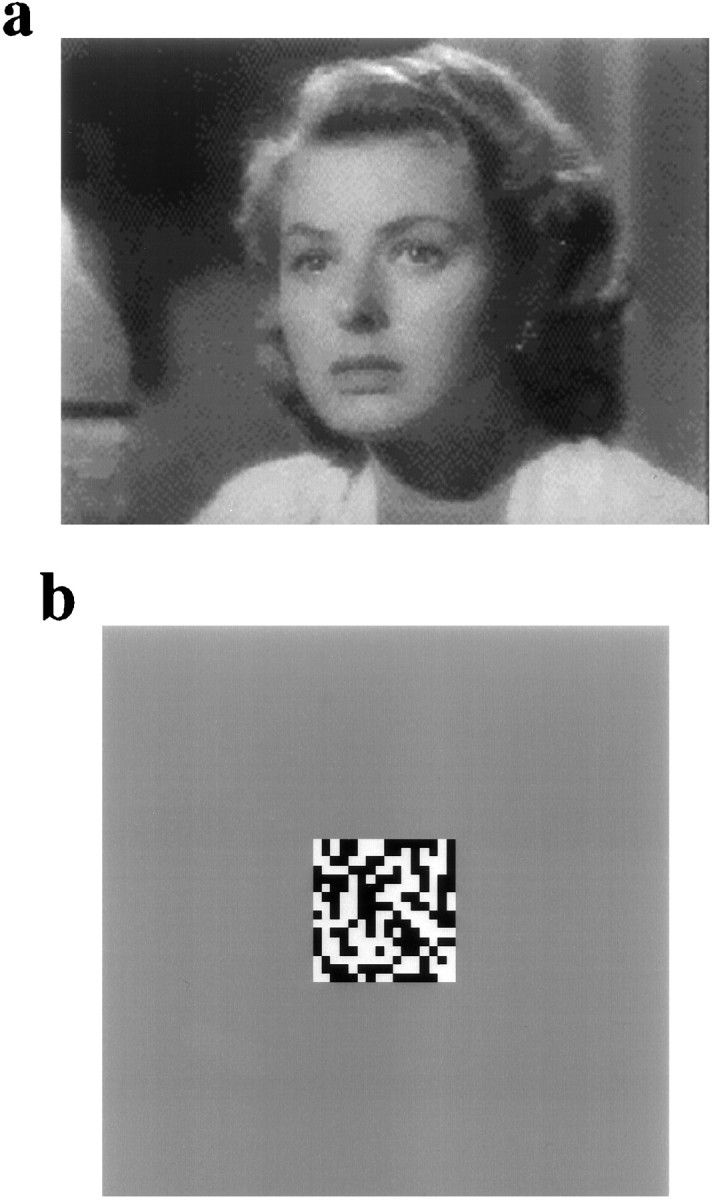
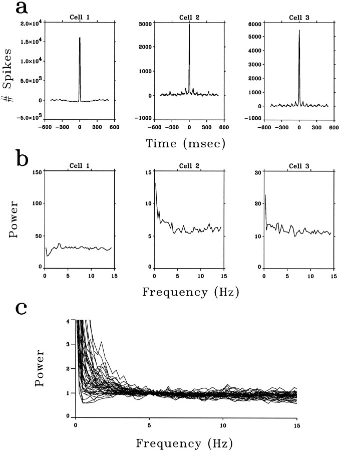
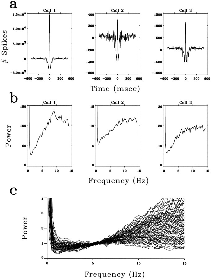
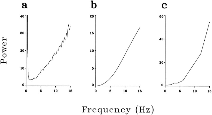
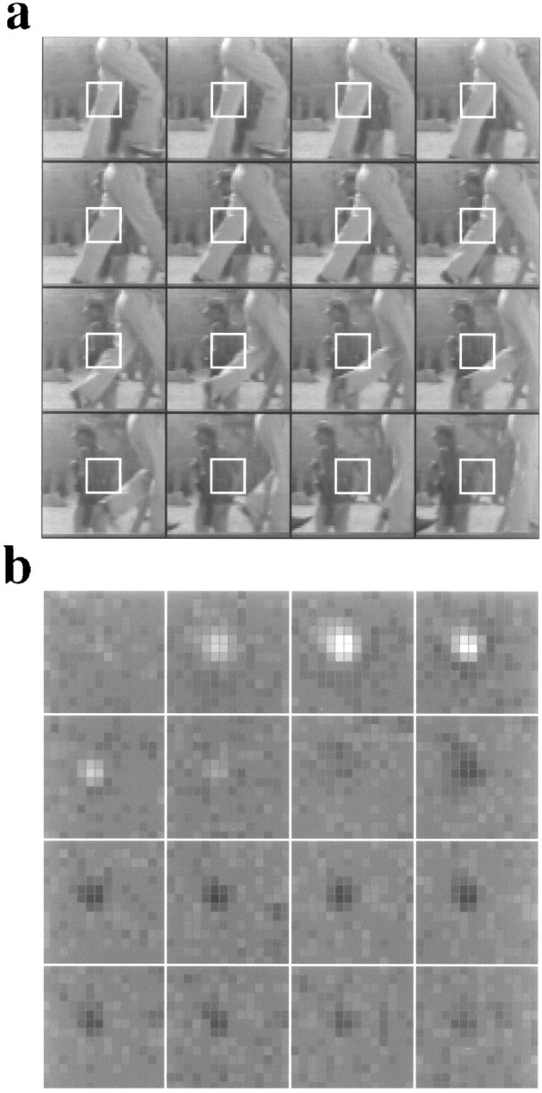
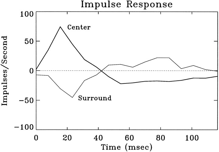
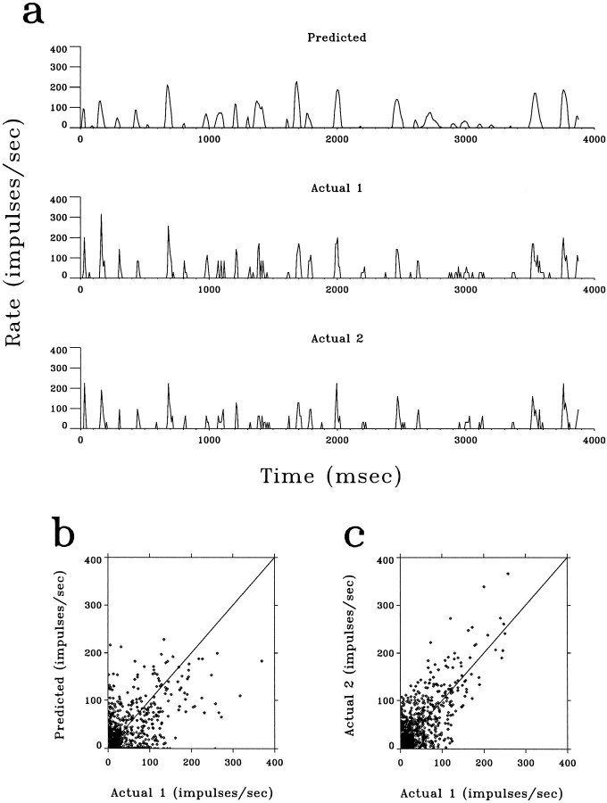
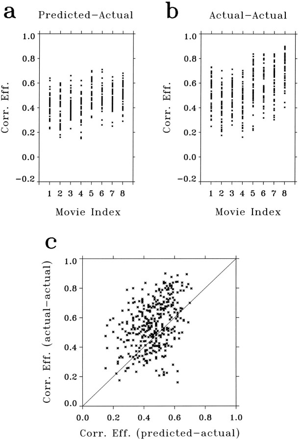
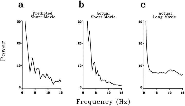
A recent computational theory suggests that visual processing in the retina and the lateral geniculate nucleus (LGN) serves to recode information into an efficient form (Atick and Redlich, 1990). Information theoretic analysis showed that the representation of visual information at the level of the photoreceptors is inefficient, primarily attributable to a high degree of spatial and temporal correlation in natural scenes. It was predicted, therefore, that the retina and the LGN should recode this signal into a decorrelated form or, equivalently, into a signal with a "white" spatial and temporal power spectrum. In the present study, we tested directly the prediction that visual processing at the level of the LGN temporarily whitens the natural visual input. We recorded the responses of individual neurons in the LGN of the cat to natural, time-varying images (movies) and, as a control, to white-noise stimuli. Although there is substantial temporal correlation in natural inputs (Dong and Atick, 1995b), we found that the power spectra of LGN responses were essentially white. Between 3 and 15 Hz, the power of the responses had an average variation of only +/-10.3%. Thus, the signals that the LGN relays to visual cortex are temporarily decorrelated. Furthermore, the responses of X-cells to natural inputs can be well predicted from their responses to white-noise inputs. We therefore conclude that whitening of natural inputs can be explained largely by the linear filtering properties (Enroth-Cugell and Robson, 1966). Our results suggest that the early visual pathway is well adapted for efficient coding of information in the natural visual environment, in agreement with the prediction of the computational theory.


Figures

Fig. 1.
Fig. 1.
Visual stimuli used in the current study: natural scenes and spatiotemporal white noise. a, A single frame from the movie Casablanca, which, together with other movies, was used as a natural stimulus. b, A single frame from spatiotemporal white noise with 100% contrast. A complete white-noise stimulus consists of 215 frames of these pseudorandom checkboard patterns.
Fig. 2.
Fig. 2.
The responses of LGN neurons evoked by natural visual stimuli. a, Autocorrelation functions of the spike trains of three LGN neurons in response to movies. The small secondary peaks for cells 2 and 3 were attributable to a weak 15 Hz artifact in the Media Player movies; see Materials and Methods. b, Power spectra of the same neurons between 0 and 15 Hz. The power spectral density is in units of (impulses/sec)2/Hz. c, Summary of the power spectra of 51 cells in response to movies. For the sake of clarity, each power spectrum is normalized by its own value at 5–6 Hz.
Fig. 3.
Fig. 3.
The responses of LGN neurons evoked by white-noise stimuli. a, Autocorrelation functions of the same LGN neurons as those shown in Figure 2, a and b, evoked by full-field white noise. b, Power spectra of these neurons. c, Summary of the power spectra of 75 LGN neurons in response to full-field white noise, normalized as described in Figure 2c. All the power spectra shown here had positive slopes. Some spectra showed small slopes, because they were less well modulated by white-noise stimuli relative to their noise levels.
Fig. 4.
Fig. 4.
Temporal-filtering properties of an LGN neuron measured with different methods. a, Power spectrum of an LGN spike train in response to full-field white noise with 100% contrast.b, The square of the Fourier transform of the temporal receptive field measured with the same full-field white noise as ina. For a perfect linear filter, this should be equivalent to the power spectrum of the response, as shown in a, except for the presence of additional noise in a. The fact thata and b have the same shape but differ in amplitude by a factor of 2 is caused largely by the rectification.c, The square of the temporal-tuning function of the same neuron. The temporal-tuning function is defined as the amplitudes of responses to sinusoidally modulated inputs with unit contrast but at different temporal frequencies. In this experiment, it was measured with spatially uniform, but temporally modulated stimuli at 25% contrast. All three functions were normalized by the power of their respective input and therefore reflect the intrinsic tuning properties of the neuron. The fact that c has a higher amplitude than both a and b suggests either a saturation in the response to 100% contrast full-field white noise or a contrast gain-control mechanism. The unit of all three power spectra is (impulses/sec)2/Hz.
Fig. 5.
Fig. 5.
Convolution of the spatiotemporal receptive fields of the LGN neurons and the short movies. a, Sixteen consecutive frames of a movie, with an interframe interval of 31.1 msec and a spatial resolution of 64 × 64 pixels. b, Receptive field of an on-center/off-surround X-cell. The 16 graphs represent the spatial receptive fields at 16 consecutive temporal frames, with an interframe interval of 7.7 msec. Each graph shows a 14 × 14 portion of the entire kernel, chosen to include both center and surround. The pixel luminance indicates the sign and magnitude of neural excitation evoked by a light signal at the position of the pixel. The magnitude of the contrast between pixels is roughly proportional to neural excitation in impulses per second. The grid separating the pixels is set to the mean luminance. The size and the signature of the surround are best appreciated by noting the large region where the receptive field is darker than the background grid (i.e., where the grid appears light). For the sake of clarity, the receptive field has been spatially magnified relative to the movie. The white squares in a indicate the areas in the images that correspond to each frame in b. To measure the actual responses, each frame in a was repeated four times so that the movie and the white-noise stimuli had the same frame rate.
Fig. 6.
Fig. 6.
Summed impulse responses for the pixels in the center and those in the surround of the receptive field shown in Figure5b. Responses were measured in terms of the average increase in the firing rate, in impulses per second, after the light phase of the stimulus. The center of the receptive field was defined by the following procedure. First, the largest single response of the spatiotemporal receptive field (as mapped with the luminance stimulus) was located. This peak defined the position of the greatest sensitivity at the optimal latency. Next, the spatial receptive field was analyzed at the peak latency. Contiguous spatial positions were included in the center if the responses were of the same sign as the strongest response and were greater than two SD above the measurement noise. The measurement noise was estimated by examining the calculated responses at long delays between stimulus and response, i.e., when any correlation was spurious. The surround was defined as all the remaining pixels (shown in the 14 × 14 portion of the entire screen).
Fig. 7.
Fig. 7.
Comparison of the predicted and theactual responses to a natural movie. a, Top trace, The predicted response of an X-cell to a movie, as calculated by convoluting the movie with the spatiotemporal receptive field of the neuron, with a subsequent rectification.Middle trace, The actual firing rate of the same neuron in response to the movie, as averaged from the responses to one set of repeats: 1, 3, 5, 7. Bottom trace, Theactual response averaged from the other set of repeats: 2, 4, 6, 8. b, The predicted (top trace in Fig.7a) versus the actual response (middle trace in Fig. 7a, Actual 1) at corresponding temporal frames.c, The response averaged from one set of repeats (2, 4, 6, 8, bottom trace, Actual 2) versus that from the interleaved set (1, 3, 5, 7, middle trace, Actual 1).
Fig. 8.
Fig. 8.
Summary of correlation coefficients between the predicted and the actual responses to natural movies. a, Scatterplot of correlation coefficients between the predicted and the actual responses to eight short movies, indexed from 1 to 8. Each point represents the data from one cell. All 49 cells studied were included in the plot. b, Correlation coefficients between the actual responses averaged from interleaved repeats (1, 3, 5, 7 vs 2, 4, 6, 8). Data from all 49 cells were included. c, Correlation coefficients shown in b versus those shown in a, for the same cells and same movies. The fact that there are more points above the diagonal line than below indicates that theactual–actual correlation is, on average, better than thepredicted–actual correlation. It is also clear from this plot that these two correlation coefficients are correlated. This suggests that the degree of correlation between the predicted and the actual responses depends largely on the noise level in the actual responses.
Fig. 9.
Fig. 9.
Linear prediction of the power spectrum in response to natural movies. a, Power spectrum of one cell in response to a short movie, calculated from the predicted firing rate.b, Power spectrum of the same cell in response to the same movie, calculated from the actual response. These spectra were not white, attributable to the imperfect statistics of the short movie. The power spectrum of the same neuron in response to a long movie is shown in c. All the power spectral-density functions are in units of (impulses/sec)2/Hz.

References

    1. Atick JJ (1992) Could information theory provide an ecological theory of sensory processing? Network: Comput Neural Sys 3:213–251. - PubMed
    1. Atick JJ, Redlich AN. Towards a theory of early visual processing. Neural Comput. 1990;2:308–320.
    1. Atick JJ, Redlich AN. What does the retina know about natural scenes? Neural Comput. 1992;4:196–210.
    1. Atick JJ, Li Z, Redlich AN. Understanding retinal color coding from first principles. Neural Comput. 1992;4:559–572.
    1. Barlow HB. Possible principles underlying the transformation of sensory messages. In: Rosenblith WA, editor. Sensory communication. MIT; Cambridge: 1961.

Publication types

LinkOut - more resources