Modeling blood flow heterogeneity

Abstract

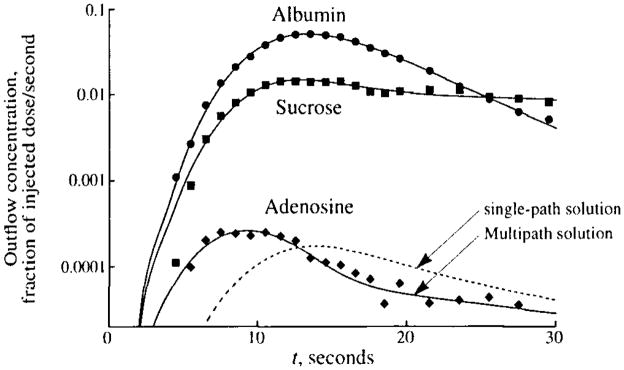
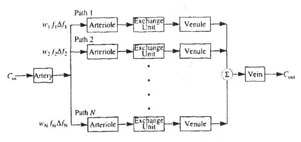
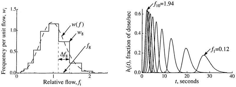
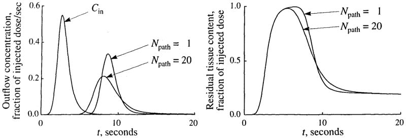
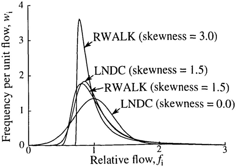
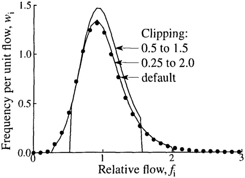
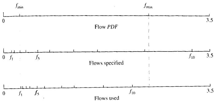
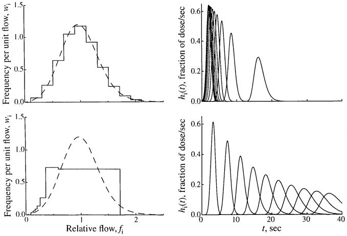
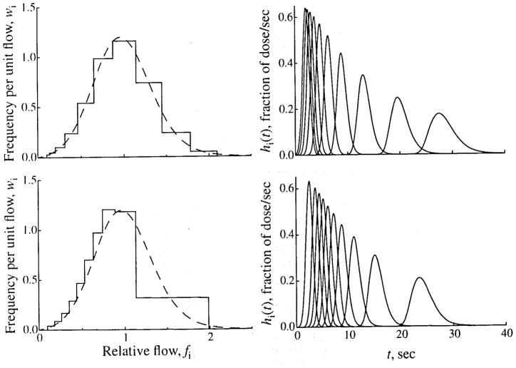
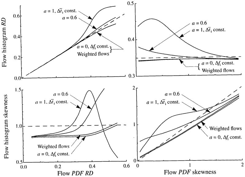
It has been known for some time that regional blood flows within an organ are not uniform. Useful measures of heterogeneity of regional blood flows are the standard deviation and coefficient of variation or relative dispersion of the probability density function (PDF) of regional flows obtained from the regional concentrations of tracers that are deposited in proportion to blood flow. When a mathematical model is used to analyze dilution curves after tracer solute administration, for many solutes it is important to account for flow heterogeneity and the wide range of transit times through multiple pathways in parallel. Failure to do so leads to bias in the estimates of volumes of distribution and membrane conductances. Since in practice the number of paths used should be relatively small, the analysis is sensitive to the choice of the individual elements used to approximate the distribution of flows or transit times. Presented here is a method for modeling heterogeneous flow through an organ using a scheme that covers both the high flow and long transit time extremes of the flow distribution. With this method, numerical experiments are performed to determine the errors made in estimating parameters when flow heterogeneity is ignored, in both the absence and presence of noise. The magnitude of the errors in the estimates depends upon the system parameters, the amount of flow heterogeneity present, and whether the shape of the input function is known. In some cases, some parameters may be estimated to within 10% when heterogeneity is ignored (homogeneous model), but errors of 15-20% may result, even when the level of heterogeneity is modest. In repeated trials in the presence of 5% noise, the mean of the estimates was always closer to the true value with the heterogeneous model than when heterogeneity was ignored, but the distributions of the estimates from the homogeneous and heterogeneous models overlapped for some parameters when outflow dilution curves were analyzed. The separation between the distributions was further reduced when tissue content curves were analyzed. It is concluded that multipath models accounting for flow heterogeneity are a vehicle for assessing the effects of flow heterogeneity under the conditions applicable to specific laboratory protocols, that efforts should be made to assess the actual level of flow heterogeneity in the organ being studied, and that the errors in parameter estimates are generally smaller when the input function is known rather than estimated by deconvolution.

FIGURE 1

Coronary sinus outflow curves for tracer albumin, sucrose, and adenosine after intracoronary bolus injection in an anesthetized, closed-chest dog with a coronary blood flow of 0.56 ml · min⁻¹ · g⁻¹. Coronary venous blood was fractionated and collected in an enzymatic stopping solution, and the deproteinated plasma was analyzed for tracer concentration using high-pressure liquid chromatography and multiple-radionuclide detection techniques. The fit of a heterogeneous flow model to the data is shown by the solid lines. The dashed line shows the best fit of a single-path model to the adenosine data. Parameter estimates are PS_C = 0.8 ml · min⁻¹ · g⁻¹, PS_pc = 1.7 ml · min⁻¹ · g⁻¹, and $V_{\text{isf}}^{\prime }=0.2\text{ml}·{\text{min}}^{-1}$ for the multipath model and PS_C = 0.5, PS_pc = 3.9, and $V_{\text{isf}}^{\prime }=0.3$ for the single-path model. (Data from 26.)

FIGURE 2

Diagram of parallel pathway model used for simulation experiments.

FIGURE 3

Relative flows and frequencies for a flow histogram with ten paths (N_path = 10). (Left) Flow PDF (dashed line), w(f), given by an LNDC with an RD of 0.35 and skewness of 0.30, and the flow histogram (solid line) constructed from it using the method of weighted flows described in Appendix A, covering the range f_min = 0.1 to f_max = 2.1. The frequency, w_i, relative flow, f_i, and width, Δf_i, of the eighth path are indicated. Both w(f) and the histogram have unity in the area and mean. (Right) The unweighted transfer functions, h_i(t), for an intravascular tracer through the individual pathways with flows specified by the flow histogram in the left panel. (LNDC input as described in Table 1.)

FIGURE 4

The effects of flow heterogeneity on tracer outflow and tissue content curves following a dispersed injection of a permeating tracer (i.e., one that diffuses across the capillary wall and permeates across cell membranes) into the inflow of an organ. The concentration-time curves are shown for the outflow concentration (left) and for the residual tissue content (right) for both homogeneous (N_path = 1) and heterogeneous (N_path = 20, flow histogram RD = 0.30) flow. The input function, C_in, is shown in the left panel. Input and model parameters are those shown in Table 1, except that PS_C was 0.25 ml · g⁻¹ · min⁻¹.

FIGURE 5

Fit of single-path model (solid line) to simulated data (symbols) generated using a 20-path model with heterogeneous flow (LNDC, RD = 30%, skewness = 0.3). The values of the parameters used to generate the data are given in Table 1. For estimated parameters, their true values and the ratios of the estimated to true values (P̂/P) are shown, as is the coefficient of variation (CV) of the model fit to the data. In fitting the data, the constraint that $V_{\text{isf}}^{\prime }+V_{\text{pc}}^{\prime }=0.8\text{ml}·{\text{g}}^{-1}$ was enforced. (Inset) Semilog plot of the tails of the curves

FIGURE 6

Estimation errors due to using a single-path model to fit multipath simulated data. Ratios of the estimates of PS_C, PS_pc, and $V_{\text{isf}}^{\prime }$ to their true values, P̂/P, with changing PS_C are shown. Simulated data were generated as in Fig. 5, with PS_C varied and PS_pc and $V_{\text{isf}}^{\prime }$ unchanged. The vertical line at PS_C = 1.0 intersects the curves at the values shown in Fig. 5.

FIGURE 7

Maps of errors in parameter estimates due to using a single-path model to fit multipath simulated data. The maps show contours of the ratio of estimated to true parameter value, P̂/P. Simulated data were generated as in Fig. 5, with different values for the membrane conductances. Shaded regions show parameter overestimates. (The dashed lines in the left panels locate the data from Fig. 6.)

FIGURE 8

The effects of incorrectly estimating flow heterogeneity on parameter estimates. P̂/P is the ratio of the estimated value to the true value of the parameter. The dashed line represents a ratio of 1.0 (i.e., no error). True values of parameters: PS_C = 1.0 ml · min⁻¹ · g⁻¹ PS_pc = 1.0 ml · min⁻¹ · g⁻¹, and $V_{\text{isf}}^{\prime }=0.16\text{ml}·{\text{g}}^{-1}$.

FIGURE 9

Fit of a single-path model to simulated data when the input function is estimated by deconvolution. (Left) The actual input function (LNDC, t̄= 3 sec, RD = 30%, skewness = 1.2) used to produce the simulated data in the right panel and the input function estimated by deconvolution. (Right) Fit of the single-path model (solid lines) to simulated data for vascular (open symbols) and permeant (filled symbols) tracers generated using a 20-path model with heterogeneous flow (LNDC, RD = 30%, skewness = 0.3). The values of the parameters used to generate the data are given in Table 1. For estimated parameters, their true values and the ratios of the estimated to true values (P̂/P) are shown, as is the coefficient of variation (CV) of the model fit to the data. In fitting the data, the input function estimated by deconvolution was used, and the constraint that $V_{\text{isf}}^{\prime }+V_{\text{pc}}^{\prime }=0.8\text{ml}·{\text{g}}^{-1}$ was enforced.

FIGURE 10

Examples of fitting simulated data with 5% noise added (symbols) for outflow and tissue content curves with heterogeneous (N_path = 20) and homogeneous (N_path = 1) models. Simulated data were generated using a 20-path model with heterogeneous flow (LNDC, flow histogram RD = 0.3, skewness = 0.3).

FIGURE 11

Probability density functions of ratios of estimated to true parameter values, P̂/P, when analyzing noisy simulated data with known flow, vascular dispersion, and input function. The simulated data had 5% noise added to the solution of a 20-path model with RD = 0.3. PDFs are shown for analysis with multipath (solid line) and single-path (dashed line) models. Vertical lines show the means of the PDFs. (Left) Analysis of outflow curves. (Right) Analysis of tissue content curves. Note that the horizontal scale of the tissue content curves is five times that used for the outflow curves.

FIGURE 12

The structure of a flow heterogeneity algorithm for calculating relative flows, f_i, and mass fractions, wd_i, from a PDF of regional flows, $f_i^{\prime },{wd}_i^{\prime }$.

FIGURE 13

Examples of lagged-normal (LNDC) and random-walk (RWALK) density functions.

FIGURE 14

The effect of clipping on the flow histogram. An LNDC with an RD of 0.35 and skewness of 1 was used for the PDF. Three levels of clipping are shown: default clipping (filled circles, relative flow limits 0.19 to 2.72), clipping at relative flows of 0.25 and 2.0 (relative flow limits 0.25 to 2.03), and maximum clipping at 0.5 and 1.5 (relative flow limits 0.52 to 1.57).

FIGURE 15

An example of the results of scaling and shifting flows specified for the flow histogram so that all flows fall within the limits of the PDF. (Top) Minimum and maximum relative flows of the flow PDF. (Center) Relative flows specified by the modeler. (Note that the first, second, and last flows are outside the range of the PDF). (Bottom) Scaled and shifted flows used for the flow histogram.

FIGURE 16

Methods of selecting relative flows for a flow histogram. (Left) Flow PDF (dashed line), w(f), given by an LNDC with an RD of 0.35 and skewness of 0.30, and the flow histogram (solid line) constructed from it, covering the range f_min = 0.1 to f_max = 2.1. (Right) The transfer functions for the individual pathways with the flows specified by the flow histogram on the left. Two methods of selecting flows are shown. In the upper panels, 10 equally spaced flows covering the range are selected. In the lower panels, 10 flows with equally spaced mean transit times are selected. Note that because of conservation constraints, the limits of the PDF are adjusted to f_min = 0.085 and f_max = 1.7.

FIGURE 17

Methods of selecting relative flows for a flow histogram. Two methods of selecting flows are shown. In the upper panels, 10 flows are selected, using the method of “weighted flows.” In the lower panels, 10 flows are selected, using a scaling factor, a, of 0.6. The left panels show the flow PDFs and histograms, and the right panels show the transfer functions of the individual pathways. (See Fig. 16 for details.)

FIGURE 18

Flow histogram RD and skewness as functions of the skewness and RD of the PDF for three levels of flow scaling, a (see Eq. 16). A 20-path model and LNDC shaped PDF were used for all curves. For the left panels, the PDF had a skewness of 1.0, and for the right panels, the PDF has an RD of 0.35.

References

1. Abounader R, Vogel J, Kuschinsky W. Patterns of capillary plasma perfusion in brains of conscious rats during normocapnia and hypercapnia. Circ Res. 1995;76:120–126. - PubMed
1. Audi SH, Krenz GS, Linehan JH, Rickaby DA, Dawson CA. Pulmonary capillary transport function from flow-limited indicators. J Appl Physiol. 1994;77:332–351. - PubMed
1. Audi SH, Linehan JH, Krenz GS, Dawson CA, Ahlf SB, Roerig DL. Estimation of the pulmonary capillary transport function in isolated rabbit lungs. J Appl Physiol. 1995;78:1004–1014. - PubMed
1. Bassingthwaighte JB, Ackerman FH, Wood EH. Applications of the lagged normal density curve as a model for arterial dilution curves. Circ Res. 1966;18:398–415. - PMC - PubMed
1. Bassingthwaighte JB. Plasma indicator dispersion in arteries of the human leg. Circ Res. 1966;19:332–346. - PMC - PubMed
Publication types
LinkOut - more resources