Decoding synapses

Abstract

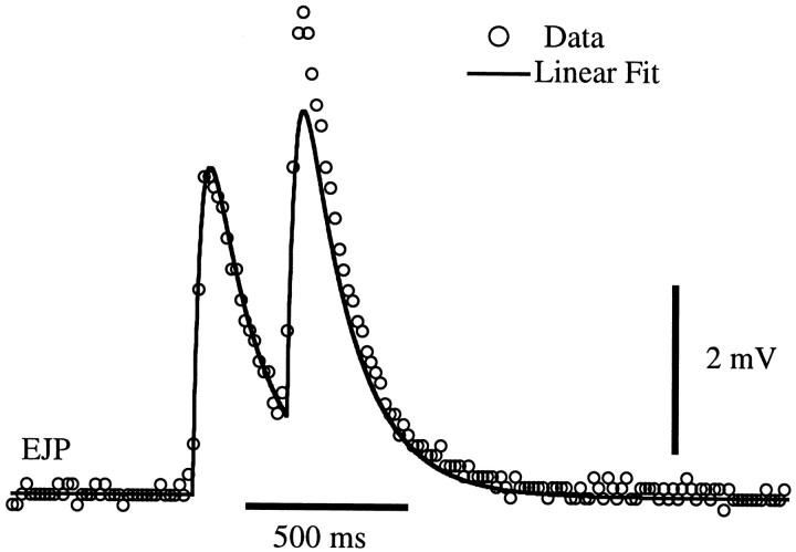
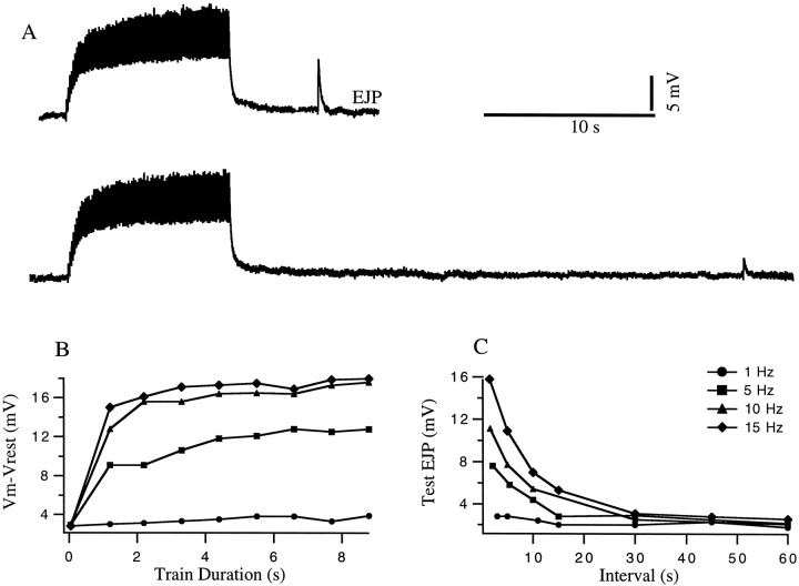
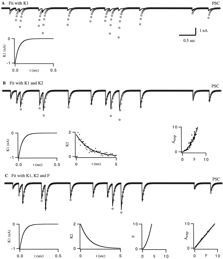
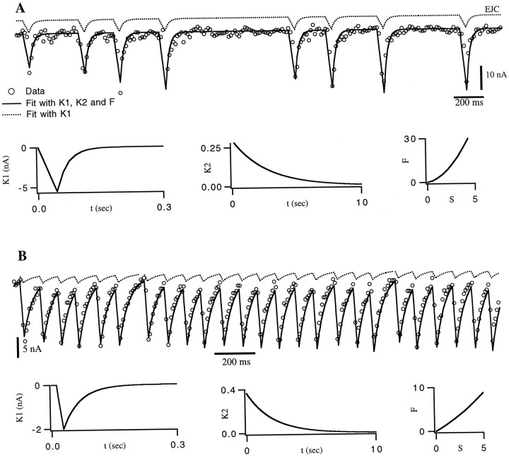
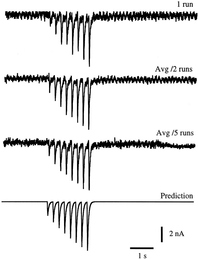
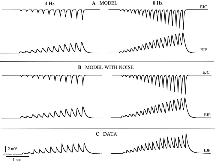
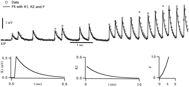
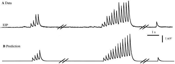
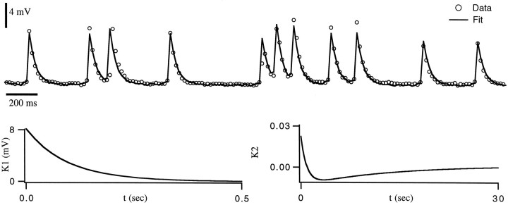
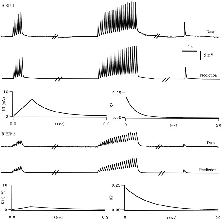
The strength of many synapses is modified by various use and time-dependent processes, including facilitation and depression. A general description of synaptic transfer characteristics must account for the history-dependence of synaptic efficacy and should be able to predict the postsynaptic response to any temporal pattern of presynaptic activity. To generate such a description, we use an approach similar to the decoding method used to reconstruct a sensory input from a neuronal firing pattern. Specifically, a mathematical fit of the postsynaptic response to an isolated action potential is multiplied by an amplitude factor that depends on a time-dependent function summed over all previous presynaptic spikes. The amplitude factor is, in general, a nonlinear function of this sum. Approximate forms of the time-dependent function and the nonlinearity are extracted from the data, and then both functions are constructed more precisely by a learning algorithm. This approach, which should be applicable to a wide variety of synapses, is applied here to several crustacean neuromuscular junctions. After training on data from random spike sequences, the method predicts the postsynaptic response to an arbitrary train of presynaptic action potentials. Using a model synapse, we relate the functions used in the fit to underlying biophysical processes. Fitting different neuromuscular junctions allows us to compare their responses to sequences of action potentials and to contrast the time course and degree of facilitation or depression that they exhibit.

Fig. 1.

Fit of EJPs by a sum of single-spike responsesK₁. Open circles show recorded EJPs evoked by a pair of spikes. The solid lineis a prediction using a linear sum of two single-spike responsesK₁. K₁ was chosen to fit single isolated spikes, and it fits the first EJP accurately. Although temporal summation is seen, the prediction based on a sum of single-spike responses fails to account for the facilitation displayed by the data. Data are from a gm8 muscle with a baseline membrane potential of −59 mV.

Fig. 2.

Conventional analysis of facilitation.A, EJPs in response to a 10 sec conditioning burst at 10 Hz followed by a test impulse 5 sec and 30 sec after the burst.B, Buildup of facilitation as a function of time for different impulse frequencies during the train. This was obtained by measuring the change in the membrane potential from rest during the 10 sec burst. Symbols are defined in C. C, Decay of facilitation as a function of time for different impulse frequencies during the train. Results were obtained by measuring the amplitude of the test EJP at various intervals after the burst. Data are from a gm8 muscle with a baseline membrane potential of −65 mV.

Fig. 3.

Fitting the response of a computational model synapse. The responses of the model are shown as open circles, and the fit is indicated by solid curves. A, The fit usingK₁ alone. This fails to capture the facilitation seen in the model. B, Fits with bothK₁ and K₂ but no nonlinearity; we have taken F = S. In this case, the fit is much better but is not perfect. The functions used are shown below the PSC plot. The middle figure is a scatter plot of the discrete point parameterization of K₂ and an exponential fit of these points. The figure at the bottom right of this panel, plotting A_exp against S, shows that the assumption F = S is not correct and suggests the form of the function F that is needed. C, Fit with K₁ andK₂ and nonlinearity F. These functions are plotted below the PSC plot. The graph at the bottom right corner of this panel compares the amplitude A_exp extracted from the data, with its prediction F.

Fig. 4.

Fit of EJCs from the gm8 muscle. In bothA and B, the upper dotted line is the result of a linear sum of single-spike responsesK₁, with no amplitude factor included. Theopen circles are data points, and the solid curve is the prediction using the functionsK₁, K₂, andF plotted in the bottom row of graphs. These fits were the end result of a gradient-descent training session based on data that included the sequence shown. A, Over the entire data set, the r.m.s. error in the prediction of the peak EJC amplitude was 1.9 nA, corresponding to a 9% relative error.B, Stimulation of another synapse at higher frequency. In this case, the r.m.s. error in the prediction of the peak EJC amplitude was 1.2 nA, corresponding to an 8% relative error.

Fig. 5.

Predicting the response to a test train. This figure uses the synapse and fit shown in Figure4A, but involves EJCs evoked by a spike train not included in the training set used in that figure. The top trace shows the actual response during one trial. Thesecond trace shows the average of EJCs evoked by two identical spike trains, and the third trace shows an average of five trials. The bottom trace is the predicted response. The prediction errors for the data shown in these cases were 0.48 nA or 10% for the top trace, 0.34 nA or 7% for the second trace, and 0.24 nA or 5% for thethird trace.

Fig. 6.

Model EJPs compared with data. A, The EJCs in response to 4 Hz and 8 Hz spike trains as predicted byK₁, K₂, and the nonlinearity of Figure 4A were fed into a simple RC model of the gm8 muscle based on measured passive properties of the muscle fiber. The resulting predicted EJPs are plotted.B, EJPs produced by the same model as inA but with added noise. C, Measured EJPs from the gm8 muscle in response to 4 Hz and 8 Hz trains.

Fig. 7.

A direct fit of EJPs for the gm8 muscle. The procedure and results are exactly like those in Figure 4 except that EJPs rather than EJCs were fit. Over the entire data set, the r.m.s. error in the prediction of the peak EJP amplitude was 0.4 mV, corresponding to a 13% relative error.

Fig. 8.

Predictions for a spike sequence not in the training set of Figure 7. The breaks in the traces represent time intervals of 20 sec and then 10 sec. A, Measured EJP response. B, The predicted response usingK₁, K₂, and the nonlinear function of Figure 7. Over the entire data set, the r.m.s. error in the prediction of the peak EJP amplitude was 0.3 mV (12% relative error).

Fig. 9.

A synapse displaying both facilitation and depression. The top trace shows the fit to the EJPs evoked by a random spike train. The functions extracted by the fitting procedure are plotted underneath the EJP trace. The nonlinear functionF is similar to that in other figures and is not plotted. Data are taken from a cpv7 muscle with a baseline potential of −63 mV. Over the entire data set, the r.m.s. error in the prediction of the peak EJP amplitude was 1.3 mV (17% relative error).

Fig. 10.

Comparison of two synapses. The breaks in the traces represent time intervals of 20 sec and then 10 sec. In both cases, the functions used for the prediction are shownunderneath the two EJP traces. Nonlinear functionsF similar to those shown in previous figures were used here but are not plotted. A, Comparison of the measured and predicted responses of a cpv4 muscle to a test spike train. The baseline membrane potential was −56 mV. Over the entire data set, the r.m.s. error in the prediction of the peak EJP amplitude was 0.7 mV (5% relative error). B, Comparison of the measured and predicted responses of a gm6 muscle to a test spike train. The baseline membrane potential was −54mV. Over the entire data set, the r.m.s. error in the prediction of the peak EJP amplitude was 0.4 mV (8% relative error).

References

1. Abbott LF. Decoding neuronal firing and modeling neural networks. Q Rev Biophys. 1994;27:291–331. - PubMed
1. Bialek W, Rieke F, de Ruyter van Steveninck RR, Warland D (1991) Reading a neural code. Science 252:1854–1857. - PubMed
1. Delaney KR, Tank DW. A quantitative measurement of the dependence of short-term synaptic enhancement on presynaptic calcium. J Neurosci. 1994;14:5885–5902. - PMC - PubMed
1. Dickinson PS. Interactions among neural networks for behavior. Curr Opin Neurobiol. 1995;5:792–798. - PubMed
1. Elson RC, Selverston AI. Mechanisms of gastric rhythm generation in the isolated stomatogastric ganglion of spiny lobsters: bursting pacemaker potentials, synaptic interactions and muscarinic modulation. J Neurophysiol. 1992;68:890–907. - PubMed
Publication types
LinkOut - more resources