Neural delays shape selectivity to interaural intensity differences in the lateral superior olive

Abstract

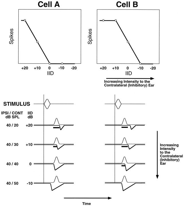
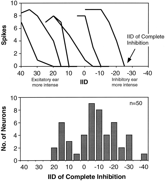
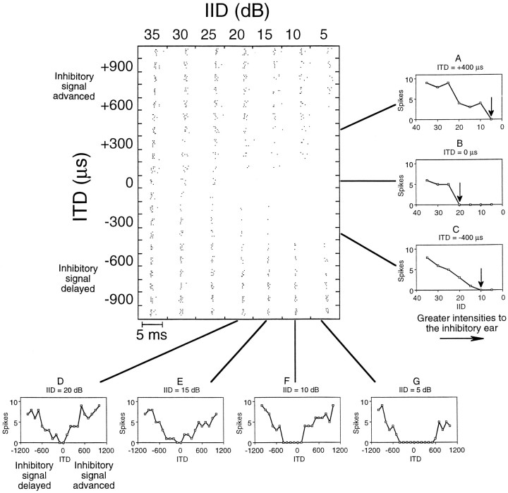
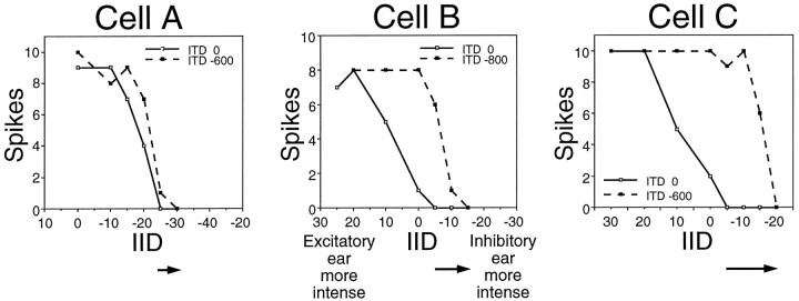
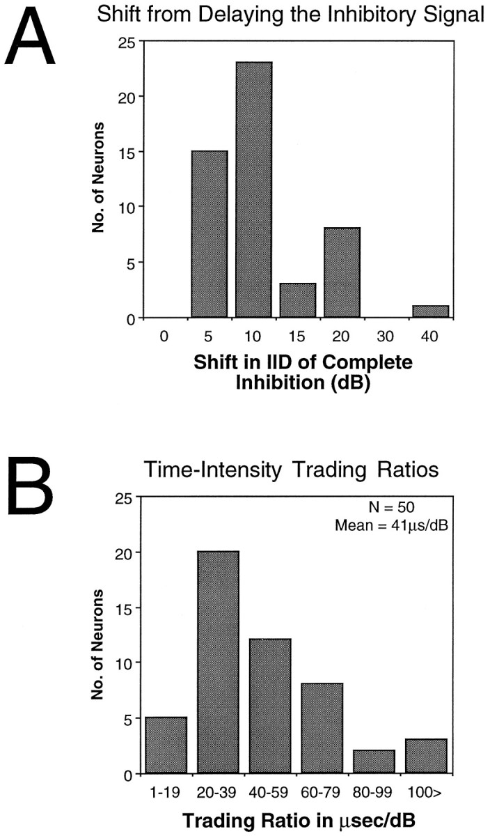
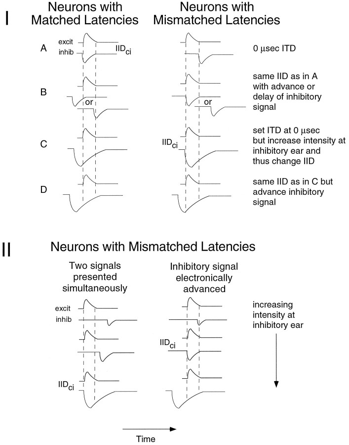
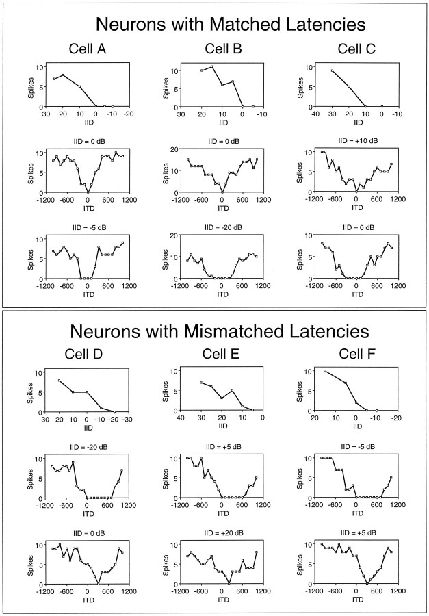
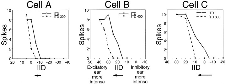
Neurons in the lateral superior olive (LSO) respond selectively to interaural intensity differences (IIDs), one of the chief cues used to localize sounds in space. LSO cells are innervated in a characteristic pattern: they receive an excitatory input from the ipsilateral ear and an inhibitory input from the contralateral ear. Consistent with this pattern, LSO cells generally are excited by sounds that are more intense at the ipsilateral ear and inhibited by sounds that are more intense at the contralateral ear. Despite their relatively homogeneous pattern of innervation, IID selectivity varies substantially from cell to cell, such that selectivities are distributed over the range of IIDs that would be encountered in nature. For some time, researchers have speculated that the relative timing of the excitatory and inhibitory inputs to an LSO cell might shape IID selectivity. To test this hypothesis, we recorded from 50 LSO cells in the free-tailed bat while presenting stimuli that varied in interaural intensity and in interaural time of arrival. The results suggest that, for more than half of the cells, the latency of inhibition was several hundred microseconds longer than the latency of excitation. Increasing the intensity to the inhibitory ear shortened the latency of inhibition and brought the timing of the inputs from the two ears into register. Thus, a neural delay of the inhibition helped to define the IID selectivity of these cells, accounting for a significant part of the variation in selectivity among LSO cells.

Fig. 1.

Model of the latency hypothesis. Top, Two IID functions from hypothetical LSO neurons illustrate different IID selectivities. Note that, compared with Cell A, Cell B responds to a wider range of IIDs. In other words, higher intensities at the inhibitory ear (more negative IIDs) are required to inhibit Cell B. Bottom, Hypothetical EPSPs and IPSPs show how the relative timing of excitation and inhibition could interact to generate different IID selectivities. In the situation shown here, IIDs from +20 to −10 dB are generated by holding the intensity to the ipsilateral (excitatory) ear constant at 40 dB SPL and varying the intensity to the contralateral (inhibitory) ear from 20 to 50 dB SPL. Theupward-deflecting curves represent excitatory postsynaptic potentials (EPSPs), whereas the downward-deflecting curvesrepresent inhibitory postsynaptic potentials (IPSPs). Bars beneath EPSP curves indicate when spikes can be evoked. For both cells, increasing the intensity to the inhibitory ear causes the latency of the IPSP to shorten, its duration to lengthen, and its strength to increase. Cell A and Cell B differ in terms of the relative timing of excitation and inhibition, and the discrepancy helps to define which IIDs can evoke spikes and which cannot (i.e., IID selectivity).

Fig. 2.

Representative IID functions and distribution of IIDs of complete inhibition for the 50 LSO neurons tested.Top, The IID functions from six cells illustrate how IID selectivity varied among the population from which we recorded. The IID of complete inhibition is indicated on one function. Bottom, Distribution of IIDs of complete inhibition for the 50 cells tested. Stimuli were 2 msec long, 10 kHz downward frequency sweeps centered at the characteristic frequency of each unit. The intensity to the ipsilateral (excitatory) ear was fixed at 20 dB above threshold, whereas the intensity to the contralateral (inhibitory) ear was varied.

Fig. 3.

Matrix of dot raster displays and selected IID and ITD functions from one LSO neuron. The matrix shows dot raster displays generated by 147 different combinations of IID and ITD. On they-axis, negative ITDs indicate that the signal to the contralateral (inhibitory) ear was delayed electronically relative to the signal to the ipsilateral (excitatory) ear, whereas positive ITDs indicate that the signal to the inhibitory ear was advanced. On thex-axis, decreasing IIDs correspond to greater intensities at the inhibitory ear. Each raster display in the matrix shows the responses to 10 presentations of the frequency sweep at one particular IID and ITD combination. The scale bar indicates the time frame for each raster display in the matrix. The characteristic frequency of this cell was 36.0 kHz, and the intensity at the excitatory ear was held constant at 50 dB SPL (20 dB above threshold). Note that the ITDs we selected to examine the timing of the neural inputs to the cell were much larger than the ITDs that the free-tailed bat would normally encounter in the free field. The small graphs show IID (A–C) and ITD (D–G) functions constructed from the spike counts along selected rows and columns of the matrix.

Fig. 4.

IID functions from three LSO cells illustrating how electronically delaying the signal to the inhibitory ear affected IID selectivity. Each graph shows the IID function of a cell when the stimulus was presented simultaneously at both ears (solid lines) and when the signal to the inhibitory ear was electronically delayed by 600 or 800 μsec relative to the signal to the excitatory ear (dashed lines). Arrows belowthe graphs indicate the magnitude of the shift for each cell. The characteristic frequencies of these cells included the following: Cell A, 49.3; Cell B, 45.0; and Cell C, 29.7 kHz; the intensity at the excitatory ear was held constant at 20 dB above threshold for each cell.

Fig. 5.

Effects of delaying the signal to the inhibitory ear on the IID of complete inhibition for the 50 LSO units tested.A, Distribution of shifts in the IID of complete inhibition.B, Distribution of time–intensity trading ratios for the 50 cells. All measures were made with the intensity at the excitatory ear fixed at 20 dB above threshold.

Fig. 6.

I, Models that illustrate differences between neurons with matched latencies and neurons with mismatched latencies.A, Timing of excitation and inhibition at an LSO cell when signals to both ears are delivered simultaneously and at intensities that evoke equally strong excitation and inhibition. With these intensities, coincidence is achieved in neurons with matched latencies, and thus this IID corresponds to the IID of complete inhibition (IID_ci). In contrast, coincidence is not achieved in neurons with mismatched latencies, and this IID does not correspond to the IID_ci. B, With the same IIDs as in A, advancing or delaying the signal to the inhibitory ear disrupts coincidence in neurons with matched latencies, but advances produce coincidence in neurons with mismatched latencies.C, Increasing the intensity at the inhibitory ear with an ITD of 0 μsec has different consequences for the two types of neurons. D, Effects of increasing the intensity of the inhibitory signal and advancing it in time. II, Left panelshows predicted effects on neurons with mismatched latencies of increasing intensity at the inhibitory ear when the two signals are presented simultaneously. Right panel shows why there should be shifts in the IID_ci for these neurons attributable to advancing the inhibitory signal in time.

Fig. 7.

Different effects of delaying or advancing the signals to inhibitory ear for three neurons with matched latencies (A–C) and for three neurons with mismatched latencies (D–F). For each cell, the top panel shows the IID function when the excitatory and inhibitory signals were presented simultaneously. The middle panel shows the ITD function generated when the intensities at the ears were set to the IID of complete inhibition. The bottom panel shows the ITD function generated with either a higher intensity to the inhibitory ear (A–C) or a lower intensity to the inhibitory ear (D–F). Positive ITDs indicate that the signal to the inhibitory ear was advanced relative to the signal at the excitatory ear. The characteristic frequencies of these cells included the following: Cell A, 45.0; Cell B, 59.5; Cell C, 31.3; Cell D, 36.9; Cell E, 35.0; and Cell F, 37.0 kHz; the intensity at the excitatory ear was held constant at 20 dB above threshold for each cell.

Fig. 8.

IID functions from three LSO cells illustrating how electronically advancing the signal to the inhibitory ear affected IID selectivity in the 27 neurons with mismatched latencies. Each graph shows the IID function of a cell when the stimulus was presented simultaneously at both ears (solid lines) and when the signal to the inhibitory ear was electronically advanced by 300 or 400 μsec relative to the signal at the excitatory ear (dashed lines). Arrows below the graphs indicate the magnitude of the shift for each cell. Each of the shifted IID functions shown represents the greatest degree of shift documented for the cell: shorter delays produced smaller shifts, whereas longer delays resulted in the functions no longer going to zero spikes. In other words, the amount by which the inhibitory signal was advanced corresponded to the point on its V-shaped ITD function, as illustrated in Figure7D–F. The characteristic frequencies of these cells included the following: Cell A, 34.5; Cell B, 21.6; and Cell C, 29.7 kHz; the intensity at the excitatory ear was held constant at 20 dB above threshold for each cell.

Fig. 9.

The distribution of shifts in the IID of complete inhibition from advancing the signal to the inhibitory ear. Thebar at 0 shift represents the 23 neurons with matched latencies, the IIDs of complete inhibition of which did not shift to less negative values. For the 27 neurons with mismatched latencies, the distribution of shifts in the IID of complete inhibition ranged from 5 to 20 dB. As in Figure 8, the shifts reported here represent the greatest degree of shift documented for each cell. All measures were made with the intensity at the excitatory ear fixed at 20 dB above threshold.

Fig. 10.

Distribution of IIDs of complete inhibition for the 27 neurons with mismatched latencies and the 23 neurons with matched latencies. IIDs of complete inhibition were measured for both populations with simultaneous stimulation of the ears, i.e., with an ITD of 0 μsec.

Fig. 11.

Schematic models showing how the matching of thresholds and latencies from the two ears could create the variety of IIDs of complete inhibition (IID_ci) in neurons with matched latencies (panels 1–3) and in neurons with mismatched latencies (panels 4–7). Each LSO cell is innervated by several fibers (arrows) from the ipsilateral (excitatory) ear and several fibers from the contralateral (inhibitory) ear. The threshold of each fiber is indicated by its position relative to the target LSO cell: fibers with high thresholds are at thetop, and fibers with progressively lower thresholds are at the bottom. The latency of the input is indicated by the distance of each fiber from the target LSO cell. For neurons with mismatched latencies, the difference between the latencies of the excitatory and inhibitory inputs is indicated by a bar that separates the LSO cell from the inputs. Shown next to each LSO cell are three hypothetical records. Each record shows the relative strength and timing of excitation (top) and inhibition (bottom) that would be generated in the LSO cell by a sound at a particular location in the frontal sound field. The top records show the excitation and inhibition resulting from a sound in the ipsilateral field that would generate an IID that favors the excitatory ear, the middle records for a sound directly in front, and the bottom record for a sound in the contralateral sound field. The location that would result in equally strong excitation and inhibition is indicated on the rightof one of the three records.

References

1. Blum JJ, Reed MC. Further studies of a model for azimuthal encoding: lateral superior olive neuron–response curves and developmental processes. J Acoust Soc Am. 1991;90:1968–1978. - PubMed
1. Boudreau JC, Tsuchitani C. Binaural interaction in the cat superior olive S-segment. J Neurophysiol. 1968;31:442–454. - PubMed
1. Caird D, Klinke R. Processing of binaural stimuli by cat superior olivary complex neurons. Exp Brain Res. 1983;52:385–399. - PubMed
1. Covey E, Vater M, Casseday JH. Binaural properties of single units in the superior olivary complex of the mustached bat. J Neurophysiol. 1991;66:1080–1094. - PubMed
1. Erulkar SD. Comparative aspects of spatial localization of sounds. Physiol Rev. 1972;52:237–360. - PubMed
Publication types
LinkOut - more resources