Virus dynamics and drug therapy

Abstract

The recent development of potent antiviral drugs not only has raised hopes for effective treatment of infections with HIV or the hepatitis B virus, but also has led to important quantitative insights into viral dynamics in vivo. Interpretation of the experimental data depends upon mathematical models that describe the nonlinear interaction between virus and host cell populations. Here we discuss the emerging understanding of virus population dynamics, the role of the immune system in limiting virus abundance, the dynamics of viral drug resistance, and the question of whether virus infection can be eliminated from individual patients by drug treatment.

Figure 1

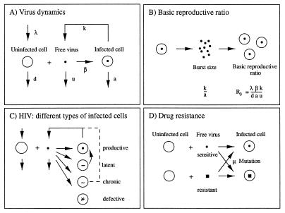
Models of virus dynamics are based on ordinary differential equations that describe the change over time in abundance of free virus, uninfected, and infected cells. (A) In the simplest model, we assume that uninfected cells, x, are produced at a constant rate, λ, and die at rate dx. Free virus is produced by infected cells at rate ky and dies at rate uv. Infected cells are produced from uninfected cells and free virus at rate βxv and die at rate ay. This leads to Eq. 1 in the text. (B) The average number of virus particles (burst size) produced from one infected cell is k/a. The basic reproductive ratio of the virus, defined as average number of newly infected cells produced from any one infected cell if most cells are uninfected (x = λ/d), is given by R₀ = (λβk)/(adu). (C) In HIV-1 infection, there are different types of infected cells. Productively infected cells have half-lifes of about 2 days and produce most (>99%) of plasma virus. Latently infected cells can be reactivated to become virus-producing cells; their turnover rate and abundance may vary among patients depending on the rate of immune activation of CD4 cells. Preliminary results suggest half-lifes of 10–20 days (21). Infected macrophages may be long-lived, chronic producers of virus particles. More than 90% of infected PBMC contain defective provirus. Their half–live was estimated to be around 80 days (2, 21). (D) The simplest models of drug resistance include a sensitive wild-type virus and a resistant mutant (Eq. 3). Mutation between wild type and mutant occurs at rate μ.

Figure 2

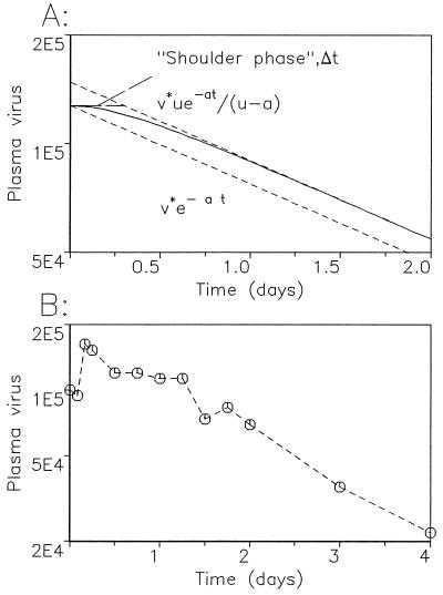
Short-term dynamics of virus decline during anti-HIV-1 treatment. (A) For a drug that reduces cell infection rates from β to sβ (s < 1), we find the amount of free virus, v(t)/v*, declines asymptotically as [Λ₂/(Λ₂ − Λ₁)]exp(−Λ₁t), where 2Λ_1,2 = (u + a) ± (providing d ≪ a, u). Thus the asymptotic slope of ln[v(t)] versus t gives a measure of Λ₁, while the duration of the shoulder phase, Δt, can be assessed from Δt = (1/Λ₁)ln(Λ₂/(Λ₂ − Λ₁)]. In the limit s → 0 (drug 100% effective), we have Λ₁ = a and Δt = (1/a)ln[u/(u − a)], for u > a. More generally, for positive s < 1 and u ≫ a, we see that the asymptotic decay rate is approximately Λ₁ ≈ a(1 − s)[1 − (sa/u) + O (a²/u²)] and the shoulder phase duration is correspondingly Δt ≈ (1/u)[1 + (a/2u)(1 − 3s) + O (a²/u²)]. (B) Plasma virus decline in a patient treated with the protease inhibitor ritonavir. Data are from ref. . Virus load starts to fall exponentially around 30 to 40 h after initiating treatment. This time span is a combination of the shoulder phase described in A, a pharmacological delay of the drug and the intracellular phase of the virus life-cycle (7, 8).

Figure 3

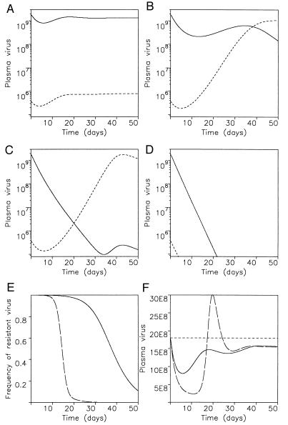
Dynamics of drug treatment if resistant virus is present before therapy. Before treatment, the basic reproductive ratios of wild-type and mutant virus are given by R₁ and R₂, respectively. Drug therapy reduces the basic reproductive ratios to R′₁ and R′₂. There are four possibilities depending on dosage and efficacy of the drug: (A) If R′₁ > R′₂, then mutant virus is still outcompeted by wild type. Emergence of resistance will not be observed. Equilibrium virus abundance during treatment is similar to the pretreatment level. (B) If R′₂ > R′₁ > 1, resistance will eventually develop, but the initial resurgence of virus can be due to wild type. (C) If R′₂ > 1 > R′₁, resistant virus rises rapidly. In B and C the exponential growth rate of resistant virus is approximately given by a(R′₂ − 1), thus providing an estimate for the basic reproductive ratio of resistant virus during treatment. (D) If 1 > R′₁, R′₂, then both wild-type and resistant virus will disappear. (E) A stronger drug will lead to a faster rise of resistant virus, if it exerts a larger selection pressure. (F) The total benefit of drug treatment, as measured by the reduction of virus load during therapy integrated over time, ∫_t (v(t) − v*)dt, is largely independent of the efficacy of the drug to inhibit wild-type replication. A stronger drug leads to a larger initial decline of virus load, but causes faster emergence of resistance. Parameter values: λ = 10⁷, d = 0.1, a = 0.5, u = 5, k₁ = k₂ = 500, β₁ = 5 × 10⁻¹⁰, β₂ = 2.5 × 10⁻¹⁰. Hence, R₁ = 10 and R₂ = 5. Treatment reduced β₁ and β₂ such that: (A) R′₁ = 3, R′₂ = 2.5; (B) R′₁ = 1.5, R′₂ = 2.25; (C) R′₁ = 0.5, R′₂ = 2; (D) R′₁ = 0.1, R′₂ = 0.5; and (E and F) R′₁ = 3, R′₂ = 4.5 (continuous line) and R′₁ = 1.5, R′₂ = 4.5 (broken line). In A–D the continuous line is wild-type virus, whereas the broken line denotes mutant.

Figure 4

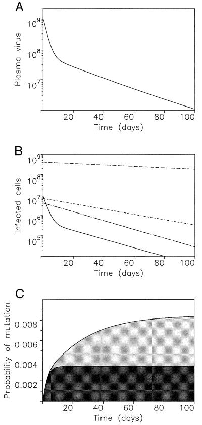
Decay of plasma virus and different types of infected cells and probability to produce resistant virus during anti-viral treatment. (A) The first phase of plasma virus decay occurs with a half-life of about 2 days and reflects the turnover rate of productively infected cells. The second phase occurs with a longer half-life (10–30 days) reflecting the decay of latently infected cells or long-lived chronic producers. (B) Productively infected cells disappear rapidly, followed by latently infected cells and chronic producers. Most infected cells may carry defective provirus and decline slowly with a half-life of about 80 days. (C) What is the probability that resistant virus is generated during therapy? Assume treatment reduces wild-type reproduction by a factor s = R′₁/R₁. Using the simplified model (2), we can calculate the total amount of mutant virus, Y₂, which is produced by mutation from wild-type virus after onset of therapy: Y₂ = ∫₀^∞ β′₁μx(τ)v₁(τ)dτ. If u ≫ a, we have v₁(t) ≈ k₁y₁/u. If a ≫ d, we have x(t) ≈ x*. During therapy y₁(t) ≈ y^*₁exp(−at). Using these approximations, we obtain Y₂ = sμy^*₁. A more accurate approximation can be obtained by assuming ẋ ≈ λ − dx during treatment (41). The probability that resistant virus exists before treatment is P₀ = 1 − exp(−y^*₂), which is for small y^*₂ approximately P₀ = y^*₂. Similarily the probability that resistant mutant is generated during therapy is P = 1 − exp(−Y₂) ≈ Y₂. Because y^*₂ > μy^*₁, we have P < sP₀. For an effective drug (small s), the probability that resistant mutant is generated during therapy is much smaller than the probability that it already existed before therapy. We can also take into account the possibility that resistant virus is generated by mutation events during production of free virus from infected cells. If this mutation rate is given by v, we find with a similar calculation that Y₂ = svy^*₁. If both mutations are possible, then Y₂ = s(μ + v)y^*₁. The mutation rates simply add up. The final result, P < sP₀, remains the same. The dark shaded area shows Y₂(t) for a simple model ignoring latency. The lighter shaded area shows the same quantity computed from a model with latency. Model equations are: uninfected cells ẋ = λ − dx − βxv; productively infected cells ẏ₁ = βq₁xv − a₁y₁ + a₂y₂; latently infected cells ẏ₂ = βq₂xv − a₂y₂; chronic producers ẏ₃ = βq₃xv − a₃y₃; defectively infected cells ẏ₄ = βq₄xv − a₄y₄; free virus v̇ = k₁y₁ + k₃y₃ − uv. Parameter values: λ = 10⁷, d = 0.1, a₁ = 0.5, a₂ = 0.05, a₃ = 0.03, a₄ = 0.008, u = 5, k₁ = 500, k₃ = 10, q₁ = 0.55, q₂ = q₃ = 0.025, q₄ = 0.4, β = 5 × 10⁻¹⁰ before therapy and β′ = 0.01β during therapy.

References

-
- Ho D D, Neumann A U, Perelson A S, Chen W, Leonard J M, Markowitz M. Nature (London) 1995;373:123–126. - PubMed
- Wei X, Ghosh S K, Taylor M E, Johnson V A, Emini E A, Deutsch P, Lifson J D, Bonhoeffer S, Nowak M A, Hahn B H, Saag M S, Shaw G M. Nature (London) 1995;373:117–122. - PubMed
- Loveday C, Kaye S, Tenant-Flowers M, Semple M, Ayliffe U, Weller I V, Tedder R S. Lancet. 1995;345:820–824. - PubMed
- Schuurman R, Nijhuis M, van-Leeuwen R, Schipper P, de Jong D, Collis P, Danner S A, Mulder J, Loveday C, Christopherson C. J Infect Dis. 1995;171:1411–1419. - PubMed
- Coffin J M. Science. 1995;267:483–489. - PubMed
Publication types
MeSH terms
Grants and funding
LinkOut - more resources
Full Text Sources