Linearity and normalization in simple cells of the macaque primary visual cortex

Abstract

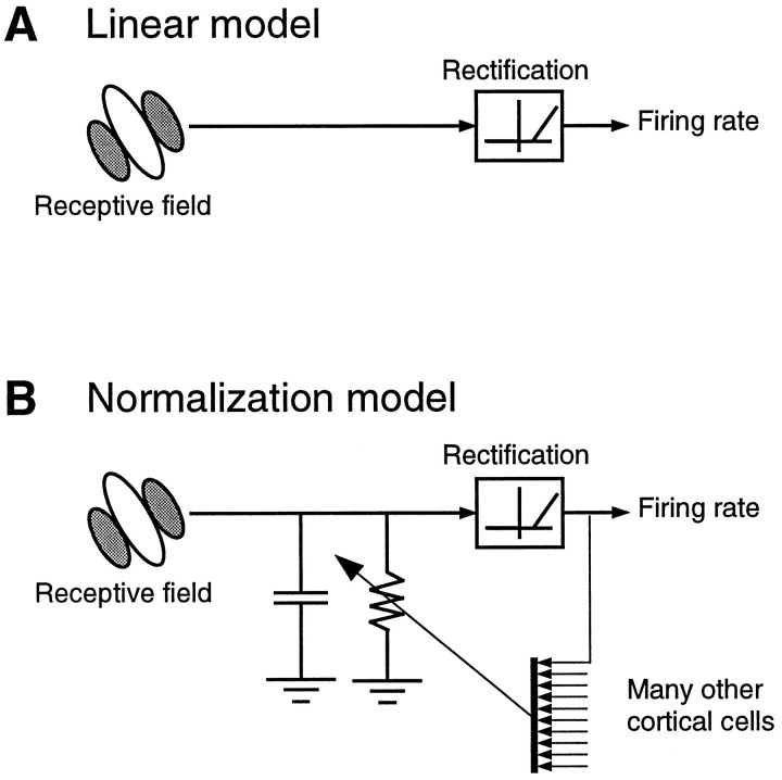
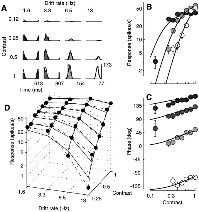
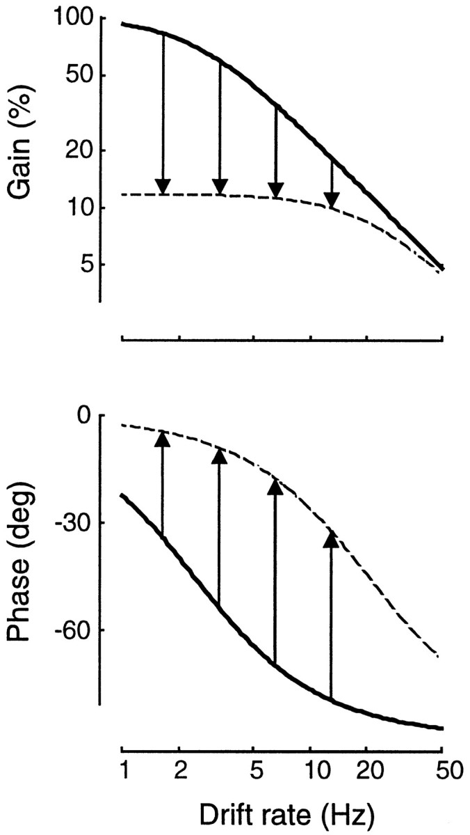
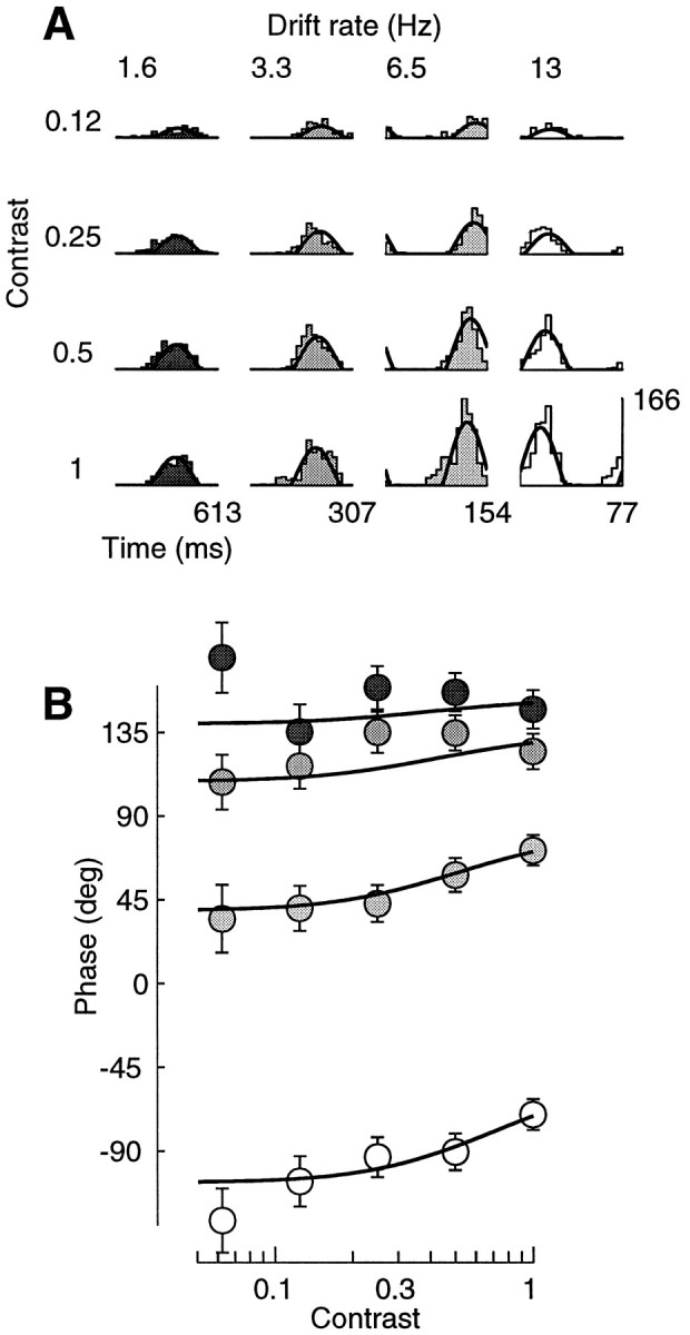
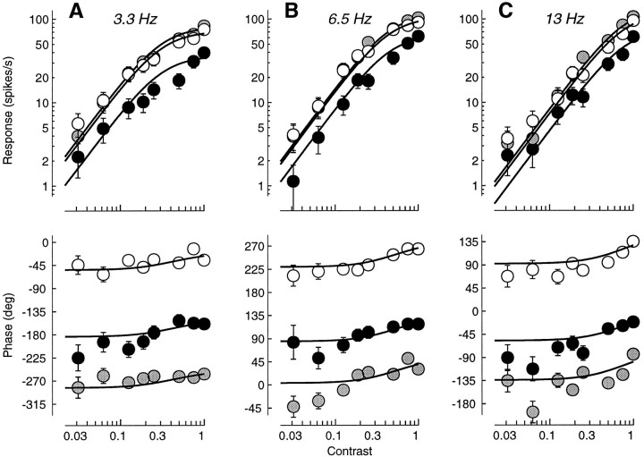
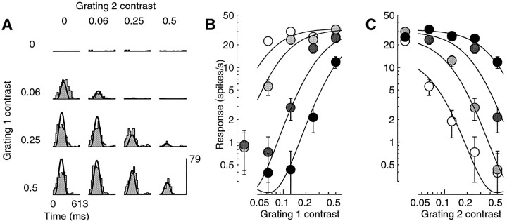
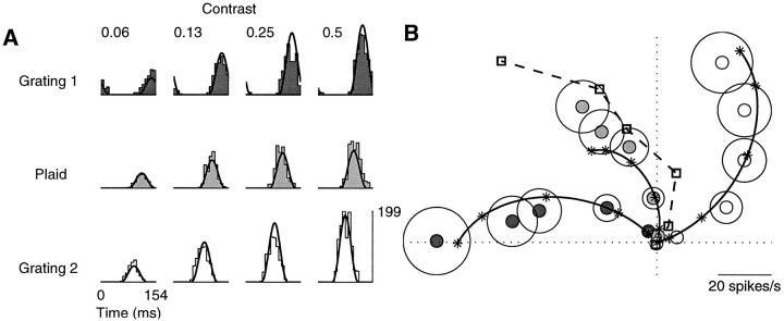
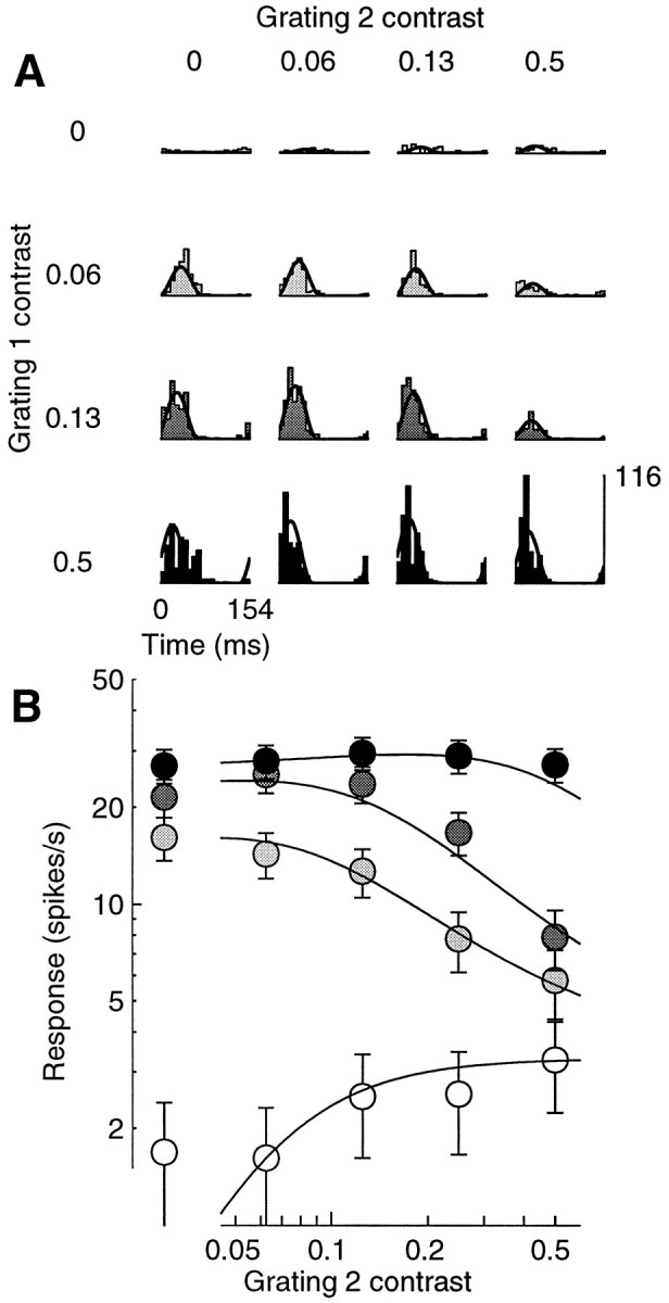
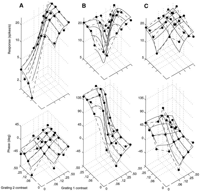
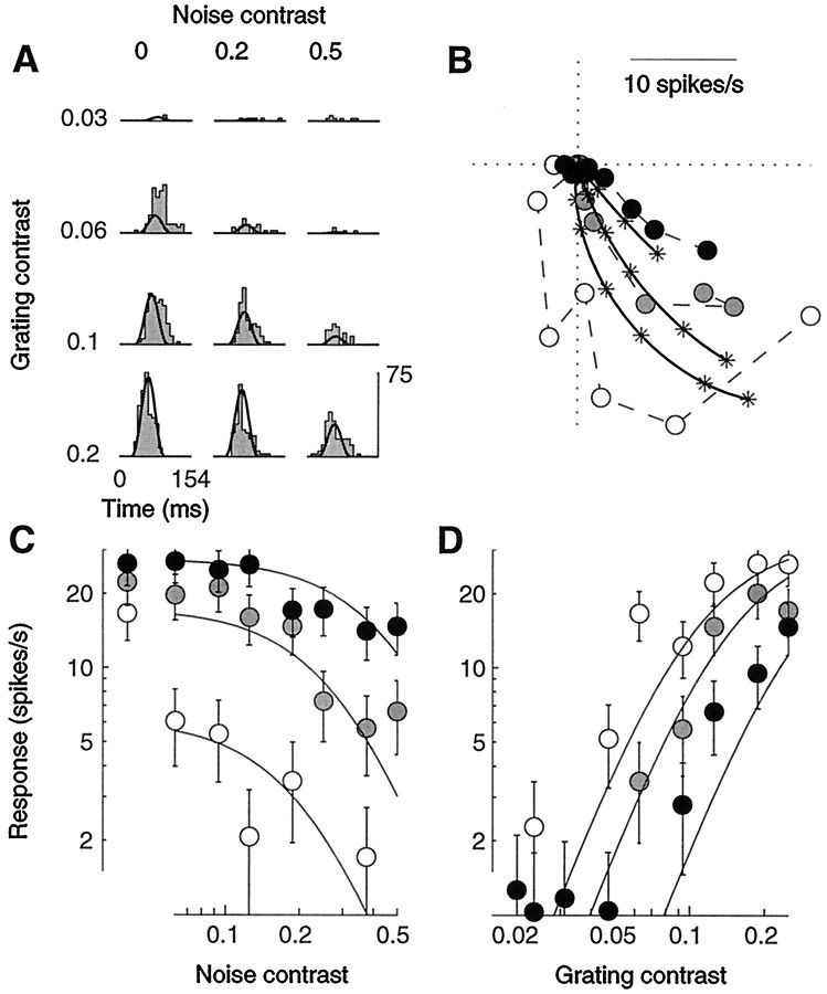
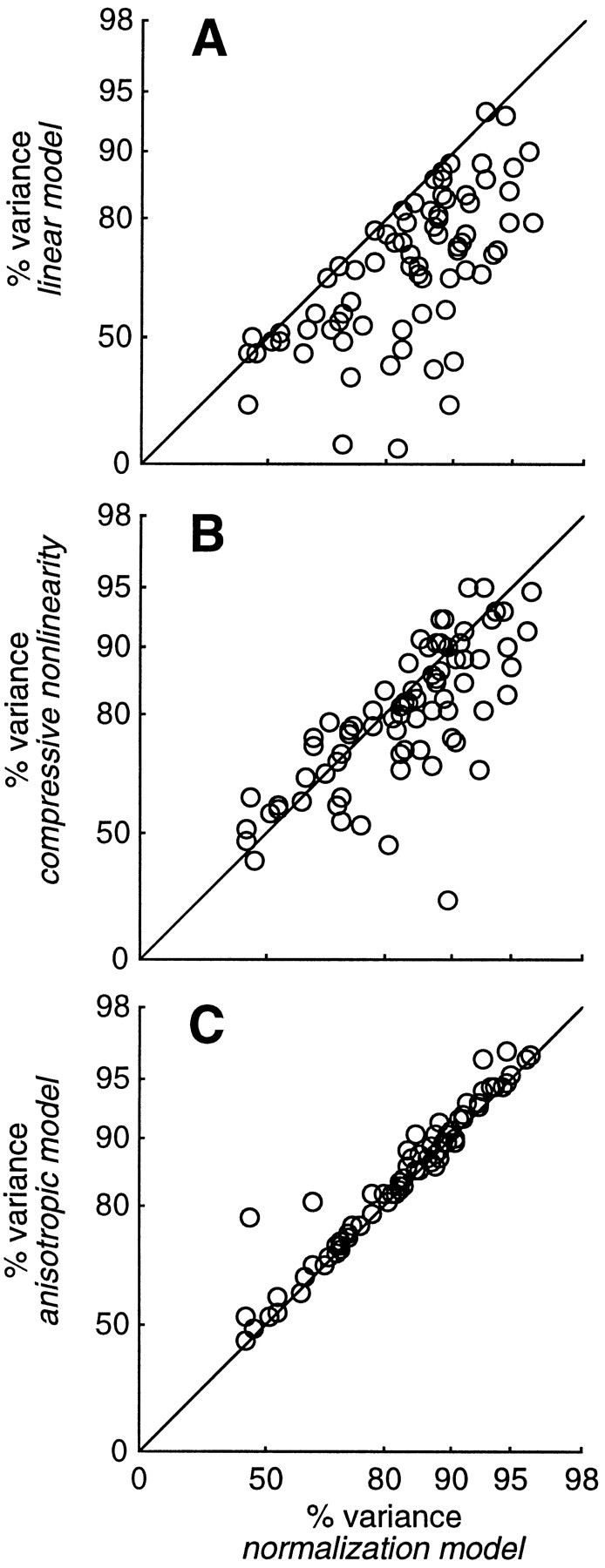
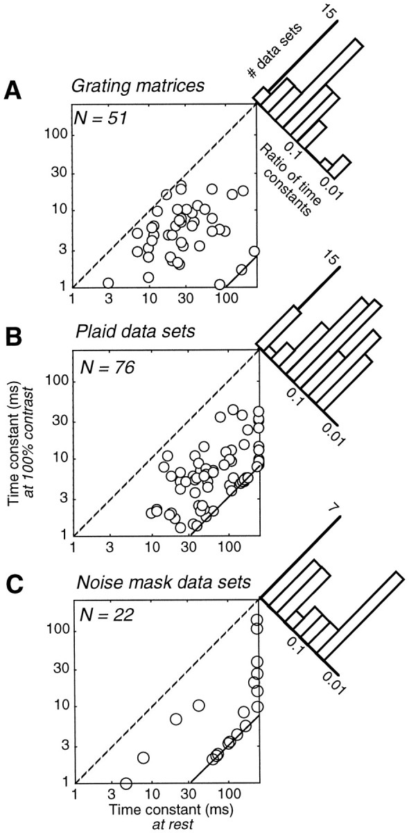
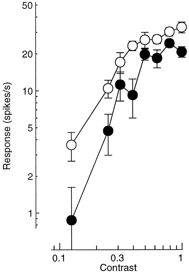
Simple cells in the primary visual cortex often appear to compute a weighted sum of the light intensity distribution of the visual stimuli that fall on their receptive fields. A linear model of these cells has the advantage of simplicity and captures a number of basic aspects of cell function. It, however, fails to account for important response nonlinearities, such as the decrease in response gain and latency observed at high contrasts and the effects of masking by stimuli that fail to elicit responses when presented alone. To account for these nonlinearities we have proposed a normalization model, which extends the linear model to include mutual shunting inhibition among a large number of cortical cells. Shunting inhibition is divisive, and its effect in the model is to normalize the linear responses by a measure of stimulus energy. To test this model we performed extracellular recordings of simple cells in the primary visual cortex of anesthetized macaques. We presented large stimulus sets consisting of (1) drifting gratings of various orientations and spatiotemporal frequencies; (2) plaids composed of two drifting gratings; and (3) gratings masked by full-screen spatiotemporal white noise. We derived expressions for the model predictions and fitted them to the physiological data. Our results support the normalization model, which accounts for both the linear and the nonlinear properties of the cells. An alternative model, in which the linear responses are subject to a compressive nonlinearity, did not perform nearly as well.

Fig. 1.

Two models of simple cell function. A, The linear model, composed of a linear stage(receptive field) and a rectification stage. The linear stage performs a weighted sum of the light intensities over local space and recent time. This sum is converted into a positive firing rate by the rectification stage. Rectification is a nonlinearity, so the “linear model” is not entirely linear. B, Thenormalization model extends the linear model by adding a divisive stage. The linear stage feeds into a circuit composed of a resistor and a capacitor in parallel (RC circuit). The conductance of the resistor grows with the pooled output of a large number of cortical cells. This effectively divides the output of the linear stage.

Fig. 2.

Interrelations and effects of the principal variables in the normalization model. A, Relation between membrane potential V and firing rate R . For simplicity in this study the resting potential is taken to be V = 0. The thick, intermediate, andthin lines depict rectification with thresholds V_thresh = 0, 6, and 12 mV, respectively. Thedashed curves indicate approximations to rectification obtained with power functions, with exponents n = 2 (thick dashes) and n = 3 (thin dashes). B, Relation between pool activity and membrane conductance. The abscissa plots the overall response of the pool, k Σ R ; the ordinate plots the increase in membrane conductance g/g₀ − 1 (Eq. 4).C, Effects of conductance on the size and time course of the membrane potential responses. The curves are the membrane potential responses to a current step with onset at time zero, for three different values of the conductance g . As the conductance doubles (thin to thick curves), it reduces both the gain and the time constant of the cell.

Fig. 3.

Responses to drifting sine gratings of different contrasts. The curves are fits of the normalization model. The fits were performed on a larger data set, which included the responses to 72 different drifting gratings (8 contrasts, 3 orientations, and 3 temporal frequencies). A, Period histograms of the responses to four different contrasts. Scale bar in spikes per second. B, C, Response amplitude and phase as a function of contrast, computed from the first harmonic of the spike trains. D, Polar plot of the responses in B andC. Every point in the plot corresponds to a sinusoid with an amplitude that is given by the distance from the origin, and the phase of which is given by the angle with the horizontal axis. As the contrast increases the responses get larger (far from the origin), and their phases advance (they turn counterclockwise). Asterisks indicate the predictions of the normalization model at the different stimulus contrasts.Circles have radius 1 SEM (N = 3) computed from the estimated variance. Error bars in B andC are ±1 SEM, computed from circles inD. Cell 392l008 [directional index (DI) = 0.1; preferred spatial frequency (SF) = 0.9 cycles/°, stimulus size (SZ) = 4.5°], experiment 4. Parameters: τ₀ = 37 msec; τ₁= 9 msec; n = 1.34.

Fig. 4.

Responses to drifting sine gratings at two different orientations, −15° (gray) and −45° (white). Fits of the normalization model (curves) were performed on a larger data set than shown, which included 72 stimulus conditions (8 contrasts, 3 orientations, and 3 temporal frequencies). A, Period histograms. Rowscorrespond to different contrasts, columns to different orientations. B, C, Response amplitude and phase as a function of contrast. To facilitate comparison in C the responses to each grating were shifted vertically so that the values predicted by the model would overlap. D, Polar plot of the responses in B and C. Cell 392l009 (DI = 0.5; SF = 0.4; SZ = 2.2), experiment 8; N = 3. Parameters: τ₀ = 28 msec; τ₁ = 3 msec;n = 1.6.

Fig. 5.

Contrast responses for gratings with two different spatial frequencies: 1.4 (gray) and 1.1 (white) cycles/degree. Fits of the normalization model (curves) were performed on a larger data set than shown, which included 40 stimulus conditions (10 contrasts, 2 spatial frequencies, and 2 temporal frequencies). Contrasts <0.12 elicited <1 spike/sec. A, Period histograms. Rows correspond to different contrasts, columns to different spatial frequencies. B, C, Response amplitude and phase as a function of contrast. Responses to each grating in C were shifted vertically so that their values predicted by the model would overlap. D, Polar plot of the responses in B andC. Cell 382l019 (DI = 0.8; SF = 1.4; SZ = 1.9), experiment 5; N = 6. Parameters: τ₀= 18 msec; τ₁ = 8 msec; n = 4.

Fig. 6.

Dependence of the contrast responses on temporal frequency. Curves are predictions of normalization model.A, Period histograms. Rows correspond to different contrasts, columns to different temporal frequencies. B, Response amplitude as a function of contrast. The 3.3 Hz data were very close to the 1.6 Hz data and were omitted to avoid clutter. C, Response phase as a function of contrast. Gray levels indicate the temporal frequency as inA. D, Response amplitude as a function of temporal frequency and contrast. Dashed lines connect actual data (dots); continuous lines indicate fits of the model. Fits were performed on a larger data set than shown, which included 64 stimulus conditions (8 contrasts, 4 temporal frequencies, and 2 orientations). Cell 382l021 (DI = 0.1; SF = 1.4; SZ = 7.5), experiment 5; N = 3. Parameters: τ₀ = 66 msec; τ₁ = 8 msec;n = 4.

Fig. 7.

Effects of changing the conductance g = 1/R in an RC circuit. Circuit parameters, and their dependence on contrast, are estimated from the experiment in Figure 6.Continuous curves show the transfer function at rest (low conductance); dashed curves show the transfer function at unit contrast (high conductance). Arrows indicate decrease in gain (top) and phase advance (bottom) at four temporal frequencies (1.6, 3.3, 6.5, and 13 Hz).

Fig. 8.

Phase advance and temporal frequency.Curves are predictions of normalization model. A, Period histograms. Rows correspond to different contrasts,columns to different temporal frequencies. B, Response phase as a function of contrast. Gray levelsindicate the temporal frequency as in A. Fits were performed on a larger data set than shown, which included 60 stimulus conditions (5 contrasts, 4 temporal frequencies, and 3 spatial frequencies). Cell 392l008 (same as Fig. 3), experiment 7; N = 3. Parameters: τ₀ = 27 msec; τ₁ = 7 msec;n = 1.2.

Fig. 9.

An entire grating matrix data set. The cell was tested with three different temporal frequencies (A, 3.3 Hz;B, 6.6 Hz; C, 13 Hz), three different orientations (white, 120°; gray, 80°;black, 40°), and nine different contrasts. Some period histograms for these responses are shown in Figure 3A. The shapes of the 18 curves are determined by only 3 parameters: τ₀ = 37 msec; τ₁ = 9 msec;n = 1.34. Eighteen additional parameters determine the vertical positions of the eighteen curves. Cell 392l008, experiment 4;N = 3.

Fig. 10.

Masking by an orthogonal grating. Responses to a plaid experiment in which one component was nearly optimally oriented (grating 1), and the other was orthogonal and ineffective in driving the cell when presented alone (grating 2). Curves are fits of the normalization model. A, Period histograms for different contrasts of the components. Rows, Different contrasts of grating 1 (c₁) .Columns, Different contrasts of grating 2 (c₂) . As c₂ was increased, the responses decreased in size (cross-orientation inhibition). B, Response amplitude as a function of c₁, for different values of c₂ (white to black: 0.06, 0.12, 0.25, and 0.5). As c₂ increased, the contrast responses shifted to the right; more and more contrast of grating 1 was needed to maintain a set level of firing. C, Same data, plotted as a function of c₂, for different values of c₁ (white toblack: 0, 0.06, 0.25, and 0.5). Cell 392l024 (DI = 0.4; SF = 0.1; SZ = 6.8), experiment 9; N = 3. Parameters: τ₀ = 158 msec; τ₁ = 5 msec;n = 2.3.

Fig. 11.

Responses to the sum of two equally effective stimuli. Components differed in spatial frequency. Continuous curves are fits of the normalization model. A, Period histograms for four different contrasts. Dark gray, Responses to grating 1 (1.2 cycles/degree). White, Responses to grating 2 (0.6 cycles/degree). Light gray, Responses to the sums of the stimuli in the top and bottom rows. B, Polar plot of the first harmonic responses.Squares indicate the vectorial sums of the responses to the individual gratings (dark gray and white data points). The actual responses to the plaid were smaller (closer to the origin) and occurred slightly sooner (counterclockwise) than this linear prediction. Cell 385r037 (DI = 0.9; SF = 0.8; SZ = 1.7), experiment 05; N = 4. Parameters: τ₀ = 45 msec; τ₁ = 2 msec;n = 2.44.

Fig. 12.

Masking with a grating that is effective in driving the cell. Responses to a plaid experiment in which one component was nearly optimally oriented (grating 1), and the other was orthogonal but still elicited some response when presented alone (grating 2). A, Period histograms for different contrasts of the components. Rows, Different contrasts of grating 1 (c₁) .Columns, Different contrasts of grating 2 (c₂) . When presented alone, grating 1 elicited strong responses (left column), grating 2 weak responses (top row). B, Response amplitude as a function of c₂, for different values of c₁ (white to black: 0, 0.06, 0.12, and 0.5). Increasing c₂ increased the size of the responses when grating 1 was absent; it inhibited the responses for intermediate contrasts of grating 1, and it had little effect for high contrasts of grating 1. Cell 392r013 (DI = 0.9; SF = 0.4; SZ = 3.4), experiment 12; N = 3. Parameters: τ₀ = 136 msec; τ₁ = 1.4 msec;n = 2.22.

Fig. 13.

Amplitude (top) and phase (bottom) of the responses of a cell to three different plaids, for different contrasts c₁ and c₂ of the two components. Circlesconnected by dashed lines are actual responses;continuous curves are fits of the normalization model. Grating 1 was the same in all three experiments. Its orientation was close to optimal. A, Grating 2 was orthogonal to grating 1.B, Grating 2 drifted 30° away from grating 1.C, Same as B, but phase of grating 2 was delayed by 90°. Cell 392r013 (same as Fig. 12), experiments 12, 9, and 8. Parameters: A, τ₀ = 40 msec; τ₁= 1.3 msec; n = 2.1; B, τ₀ = 35 msec; τ₁ = 1.4 msec; n = 1;C, τ₀ = 52 msec; τ₁ = 1.7 msec;n = 1.1.

Fig. 14.

Masking with spatiotemporal white noise. An optimal drifting grating was presented together with full-screen two-dimensional flickering binary noise. Fits of the normalization model (curves) were performed on a larger data set than shown, which included 72 stimulus conditions (9 grating contrasts and 8 mask contrasts). A, Period histograms for different grating contrasts (rows) and noise contrasts (columns). When presented alone, the grating elicited strong responses (left column), the noise very weak responses (top row).B, Polar plot of the contrast responses for three different noise contrasts (white to black: 0, 0.19, and 0.5). Increasing noise contrast decreased response amplitude and advanced response phase. Error circles are omitted to avoid clutter but can be estimated from following panels. C, Response amplitude as a function of noise contrast. Grating contrasts (white to black): 0.06, 0.12, and 0.25.D, Response amplitude as a function of grating contrast, for different noise contrasts. Gray levels as in B. Cell 394l015 (DI = 0.6; SF = 2.3; SZ = 6.8° for the stimulus, 7.8° for the mask), experiment 7. Parameters: τ₀ = 82 msec; τ₁ = 2.6 msec;n = 1.85.

Fig. 15.

Performance of four different models, measured by the percentage of the variance accounted for in the data. Eachdata point corresponds to a plaid experiment. Theabscissas plot the performance of the normalization model, and the ordinates plot performance of three other models.A, Linear model. B, Compressive nonlinearity model. C, Anisotropic model.

Fig. 16.

Time constants of V1 simple cells estimated by the normalization model from grating matrix data sets (A), from plaid data sets (B), and from noise masking data sets (C). Scatter diagrams plot the time constant at rest τ₀(abscissa) versus the time constant at full contrast τ₁ (ordinate). Time constants <1 msec are omitted. Dashed line indicates the identity τ₀= τ₁. Continuous lines in lower right corners indicate bounds in fitting procedure.Histograms show the distribution of ratios τ₁/τ₀. These include data sets with both time constants <1 msec that are missing from scatter diagrams.

Fig. 17.

An example of response variability across experiments. Data points represent responses of the same cell to the same stimuli in two different experiments. Stimuli were gratings drifting at 3.3 Hz. Error bars represent 1 SEM. The first experiment (black) involved a block of 40 stimuli (10 contrasts, 2 temporal frequencies, and 2 spatial frequencies;N = 6). The second experiment (white) was initiated 58 min after the first and involved a block of 90 stimuli (10 contrasts, 3 orientations, and 3 temporal frequencies;N = 5). Unit 389l019, experiments 5 and 6.

Fig. 18.

Saturation and phase advance for all the data sets in this study, estimated (at 6.5 Hz) from the fits of the normalization model. White, Grating matrix data sets.Black, Noise-masking data sets. Gray, Plaid data sets. The abscissa shows the saturation index: values of ≤1 indicate little or no saturation (see text). The ordinateshows the total phase advance between 0 and unit contrast.

References

1. Adelson EH, Bergen JR. Spatiotemporal energy models for the perception of motion. J Opt Soc Am A. 1985;2:284–299. - PubMed
1. Albrecht DG. Visual cortex neurons in monkey and cat: effect of contrast on the spatial and temporal phase transfer functions. Vis Neurosci. 1995;12:1191–1210. - PubMed
1. Albrecht DG, Geisler WS. Motion sensitivity and the contrast-response function of simple cells in the visual cortex. Vis Neurosci. 1991;7:531–546. - PubMed
1. Albrecht DG, Hamilton DB. Striate cortex of monkey and cat: contrast response function. J Neurophysiol. 1982;48:217–237. - PubMed
1. Albrecht DG, Farrar SB, Hamilton DB. Spatial contrast adaptation characteristics of neurones recorded in the cat’s visual cortex. J Physiol (Lond) 1984;347:713–739. - PMC - PubMed
Publication types
LinkOut - more resources