Spatial relationships among three columnar systems in cat area 17

Abstract

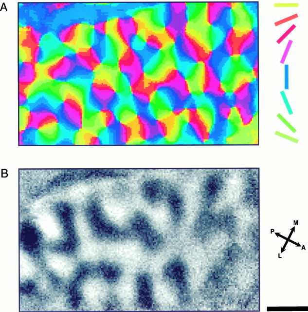
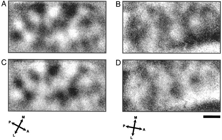
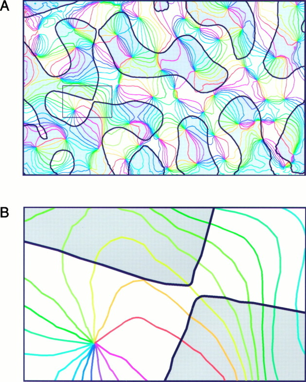
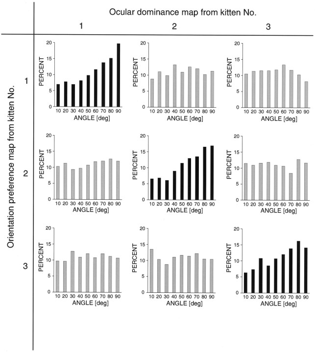
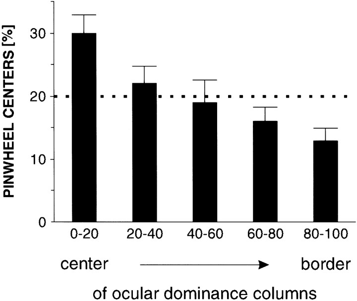
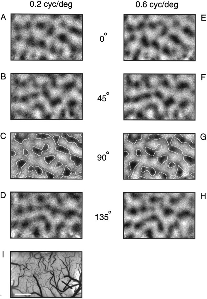
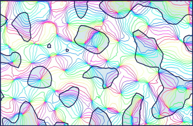
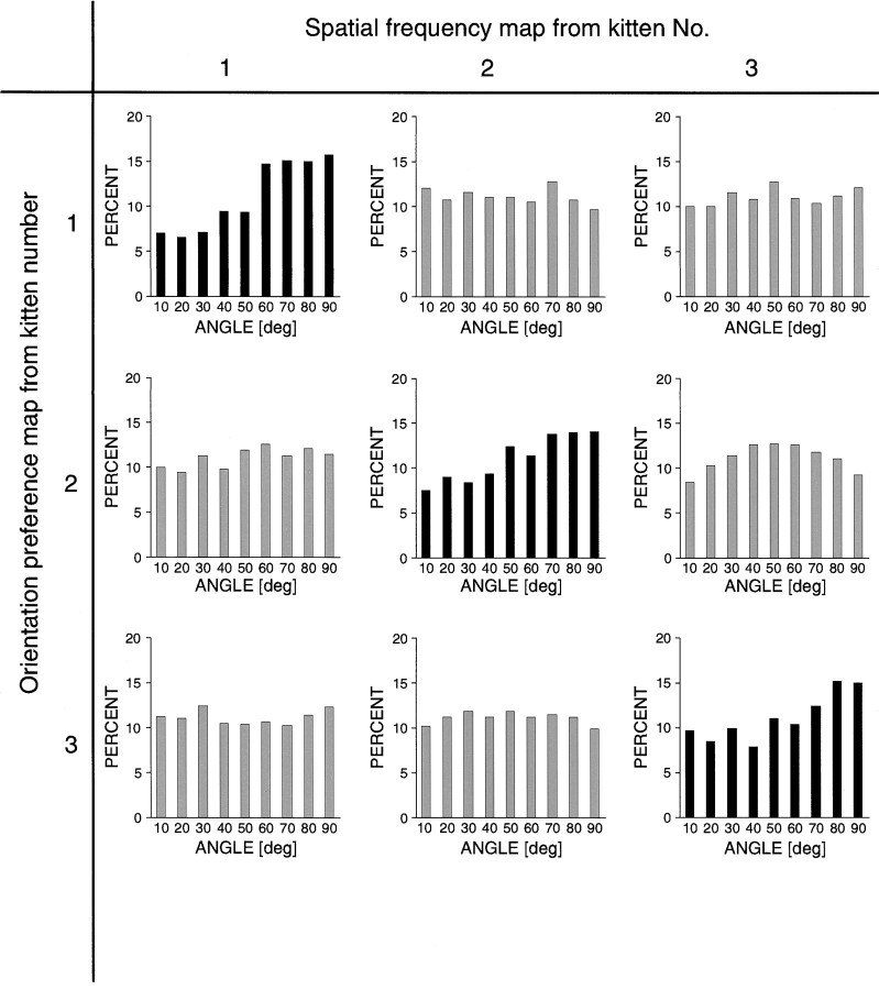
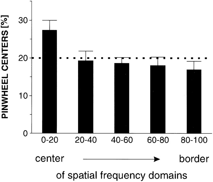
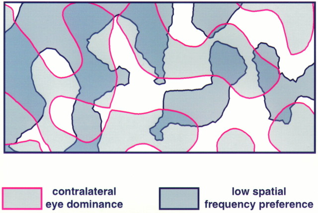
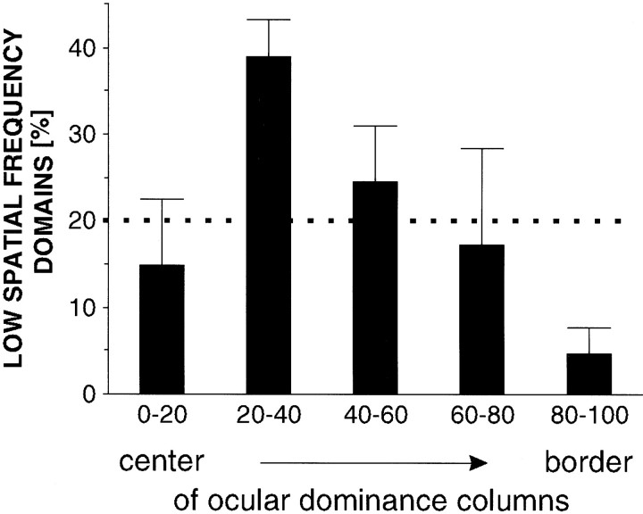
In the primary visual cortex, neurons with similar response properties are arranged in columns. As more and more columnar systems are discovered it becomes increasingly important to establish the rules that govern the geometric relationships between different columns. As a first step to examine this issue we investigated the spatial relationships between the orientation, ocular dominance, and spatial frequency domains in cat area 17. Using optical imaging of intrinsic signals we obtained high resolution maps for each of these stimulus features from the same cortical regions. We found clear relationships between orientation and ocular dominance columns: many iso-orientation lines intersected the borders between ocular dominance borders at right angles, and orientation singularities were concentrated in the center regions of the ocular dominance columns. Similar, albeit weaker geometric relationships were observed between the orientation and spatial frequency domains. The ocular dominance and spatial frequency maps were also found to be spatially related: there was a tendency for the low spatial frequency domains to avoid the border regions of the ocular dominance columns. This specific arrangement of the different columnar systems might ensure that all possible combinations of stimulus features are represented at least once in any given region of the visual cortex, thus avoiding the occurrence of functional blind spots for a particular stimulus attribute in the visual field.

Fig. 1.

Monocular stimulation of the contra- and ipsilateral eye produces different activity patterns in cat area 17.A–H, Iso-orientation maps obtained after monocular stimulation with gratings of four different orientations. Thedark patches denote regions that were activated by the respective stimulus. Active regions in the contralateral 135° map shown in D were outlined and transferred to the corresponding ipsilateral map in H to facilitate comparison. Both maps are clearly different, thus suggesting also a segregation according to ocular dominance. I, Cortical blood vessel pattern of the imaged region. A, Anterior;P, posterior; M, medial;L, lateral. Scale bar, 1 mm.

Fig. 2.

Orientation preference “angle map” and ocular dominance map from the same patch of cortex. A, Orientation preference map calculated from the iso-orientation maps shown in Figure 1. The angle of the preferred orientation is color-coded according to the key shown on the right. As described previously, orientation domains are organized in a pinwheel-like manner. B, Ocular dominance map. Blackcodes for contralateral and white for ipsilateral eye preference. The layout of the ocular dominance map is clearly different from that of the iso-orientation maps shown in Figure 1. Scale bar, 1 mm.

Fig. 3.

Variability in the width and shape of ocular dominance bands between animals. A, B, Ocular dominance maps from two additional cats. Black regions were activated stronger by the contralateral eye. Compared with the map shown in Figure 2, the spacing of the columns is wider, and the overall layout seems to be more irregular.C, D, The same maps as shown inA and B, respectively, but now with a reversed gray scale: black regions were activated stronger by the ipsilateral eye. The coding was reversed to facilitate comparison between regions activated by the contra- and ipsilateral eye. There do not seem to be strong differences between the size of the cortical representations of the two eyes. Scale bar, 1 mm.

Fig. 4.

Relationship between ocular dominance and orientation maps. A, The colored iso-orientation lines were derived from the orientation preference map shown in Figure 2. All points on lines with a given color prefer the same orientation. The contours of the ocular dominance columns were obtained from the ocular dominance map of the same cortical region, using an objective automated procedure; gray denotes contralateral eye dominance. On closer inspection it becomes clear that both systems are spatially related: many iso-orientation lines cross the borders between ocular dominance columns close to right angles, and the pinwheel-centers are preferentially located in the middle of the ocular dominance columns.B, Enlarged detail from A (seesmall rectangle on the left side of the map), showing that the tendency for perpendicular intersections is maintained even in regions where the ocular dominance bands make sharp turns.

Fig. 5.

Quantitative analysis of intersection angles between iso-orientation lines and ocular dominance borders. Nine histograms are shown in the form of a 3 × 3 matrix. The black histograms along the diagonal show the distribution of intersection angles from three cats. In all cases there is a clear predominance of large intersection angles. Each of the gray histogramsoff the diagonal was computed by overlaying an orientation map from one cat with an ocular dominance map from a different cat. In these control cases the distributions are nearly flat.

Fig. 6.

Relative frequency of pinwheel-centers in different subregions of ocular dominance maps. The maps (n = 6) were divided into five regions of equal area, with the 0–20 percentile denoting the center and the 80–100 percentile denoting the border regions of the ocular dominance columns (error bars are SEM). The dotted line indicates the expected value (20%) if the pinwheel-centers were distributed randomly. There is a high incidence of pinwheel-centers in the center regions of the ocular dominance columns.

Fig. 7.

Stimulation with different spatial frequencies causes different activity patterns. A–H, Iso-orientation maps obtained after stimulation with oriented gratings at a low (0.2 cycles/degree) and a high (0.6 cycles/degree) spatial frequency. At a given orientation the low and high spatial frequency maps are similar, but not identical (see outlines from the map inC, copied to the map in G).I, Cortical blood vessel pattern. Scale bar, 1 mm.

Fig. 8.

Stimulus preference maps derived from the iso-orientation maps shown in Figure 7. A, Orientation preference map. B, Spatial frequency map. Dark patches were activated by low spatial frequencies, and lighter regions preferred high spatial frequencies. Note that the low spatial frequency patches tend to form islands in a matrix of high spatial frequency preference. Scale bar, 1 mm.

Fig. 9.

Relationship between spatial frequency and orientation maps. The iso-orientation lines and contours of the spatial frequency domains were obtained from the maps shown in Figure 8;gray regions preferred low spatial frequencies. Scrutiny of this image reveals that the iso-orientation lines tend to cross the borders between spatial frequency domains at right angles, and that the pinwheel-centers are often located in the centers of either low or high spatial frequency domains.

Fig. 10.

Intersection angles of iso-orientation lines with borders between spatial frequency domains. Nine histograms are shown in the form of a 3 × 3 matrix. The black histogramsalong the diagonal show the distribution of intersection angles from three kittens. Large angles (black histograms) are clearly over-represented, whereas this is not the case in the controls (gray histograms).

Fig. 11.

Relative frequency of pinwheel-centers in different regions of spatial frequency maps (n = 13). Same conventions as in Figure 6. Pinwheel-centers are found more often in the center regions than near the borders of spatial frequency domains.

Fig. 12.

Relationship between ocular dominance and spatial frequency domains. In this overlay contralateral eye dominance is coded by light gray with red outlines, and low spatial frequency is coded by dark gray withblack outlines. No obvious spatial relationships are discernible at a first glance. Quantitative analysis, however, reveals that the centers of low spatial frequency domains tend to avoid the borders of the ocular dominance columns (see Fig. 13).

Fig. 13.

Frequency of centers of low spatial frequency domains in different regions of ocular dominance maps (n = 6). Same conventions as in Figure 6. Only very few low spatial frequency domains (and thus blobs) are centered on the border regions of ocular dominance columns.

References

1. Anderson PA, Olavarria J, Van Sluyters RC. The overall pattern of ocular dominance bands in cat visual cortex. J Neurosci. 1988;8:2183–2200. - PMC - PubMed
1. Bartfeld E, Grinvald A. Relationships between orientation preference pinwheels, cytochrome oxidase blobs and ocular dominance columns in primate striate cortex. Proc Natl Acad Sci USA. 1992;89:11905–11909. - PMC - PubMed
1. Berardi N, Bisti S, Cattaneo A, Fiorentini A, Maffei L. Correlation between the preferred orientation and spatial frequency of neurones in visual areas 17 and 18 of the cat. J Physiol (Lond) 1982;323:603–618. - PMC - PubMed
1. Blasdel GG. Differential imaging of ocular dominance and orientation selectivity in monkey striate cortex. J Neurosci. 1992;12:3115–3138. - PMC - PubMed
1. Blasdel GG, Salama G. Voltage-sensitive dyes reveal a modular organization in monkey striate cortex. Nature. 1986;321:579–585. - PubMed
Publication types