Feature extraction by burst-like spike patterns in multiple sensory maps

Abstract

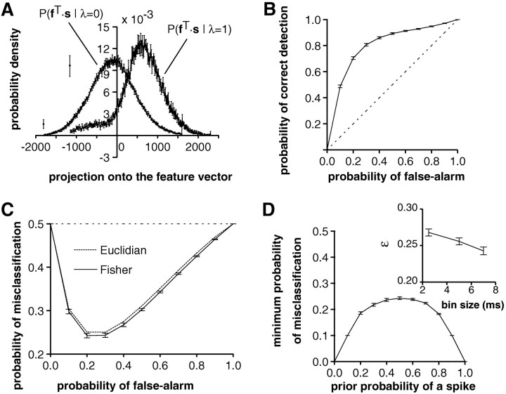
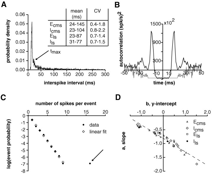
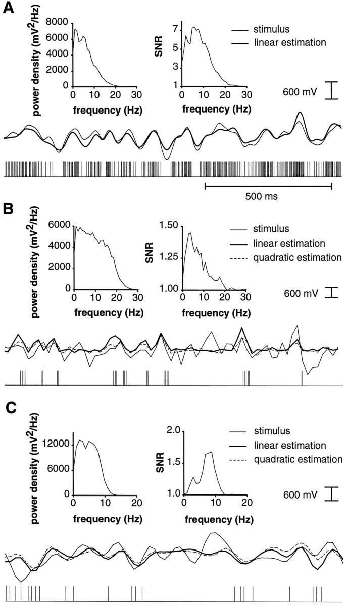
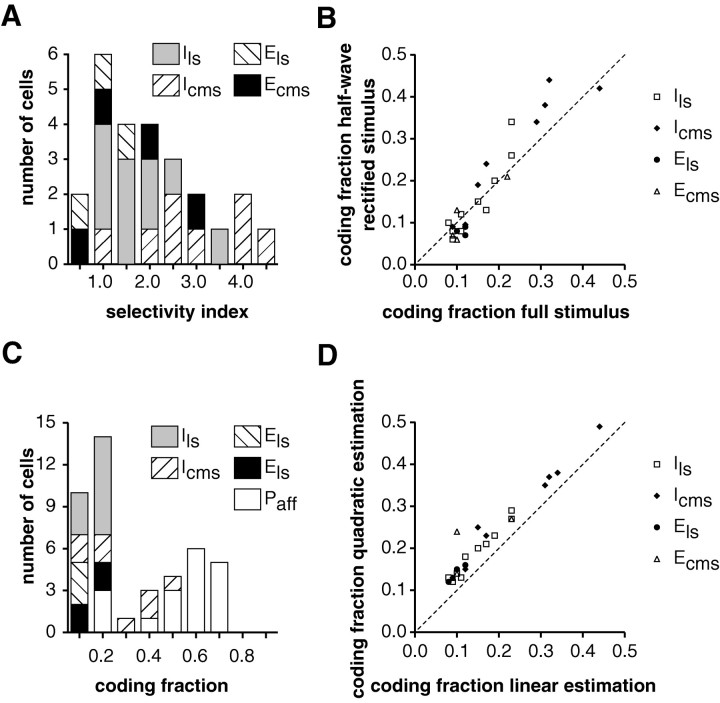
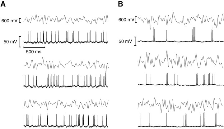
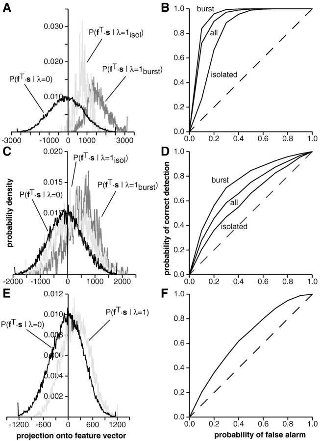
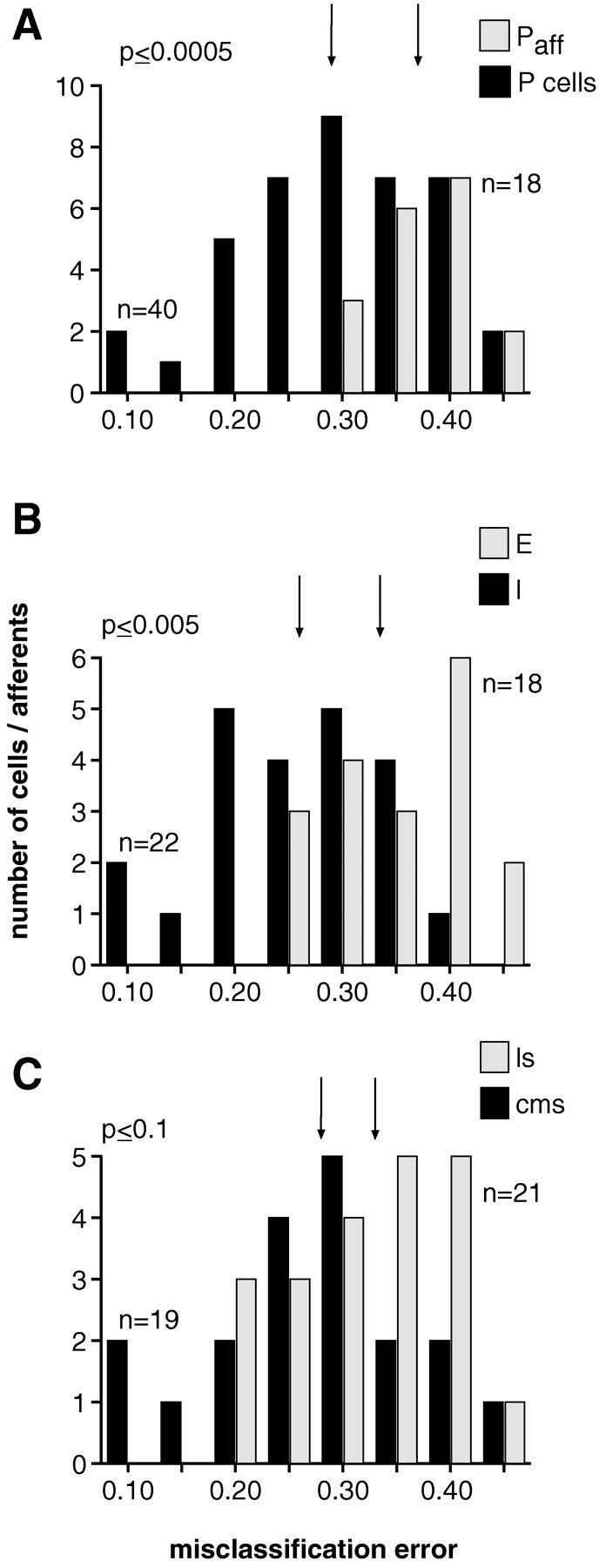
In most sensory systems, higher order central neurons extract those stimulus features from the sensory periphery that are behaviorally relevant (e.g.,Marr, 1982; Heiligenberg, 1991). Recent studies have quantified the time-varying information carried by spike trains of sensory neurons in various systems using stimulus estimation methods (Bialek et al., 1991; Wessel et al., 1996). Here, we address the question of how this information is transferred from the sensory neuron level to higher order neurons across multiple sensory maps by using the electrosensory system in weakly electric fish as a model. To determine how electric field amplitude modulations are temporally encoded and processed at two subsequent stages of the amplitude coding pathway, we recorded the responses of P-type afferents and E- and I-type pyramidal cells in the electrosensory lateral line lobe (ELL) to random distortions of a mimic of the fish's own electric field. Cells in two of the three somatotopically organized ELL maps were studied (centromedial and lateral) (Maler, 1979; Carr and Maler, 1986). Linear and second order nonlinear stimulus estimation methods indicated that in contrast to P-receptor afferents, pyramidal cells did not reliably encode time-varying information about any function of the stimulus obtained by linear filtering and half-wave rectification. Two pattern classifiers were applied to discriminate stimulus waveforms preceding the occurrence or nonoccurrence of pyramidal cell spikes in response to the stimulus. These signal-detection methods revealed that pyramidal cells reliably encoded the presence of upstrokes and downstrokes in random amplitude modulations by short bursts of spikes. Furthermore, among the different cell types in the ELL, I-type pyramidal cells in the centromedial map performed a better pattern-recognition task than those in the lateral map and than E-type pyramidal cells in either map.

Fig. 1.

A, Frontal section through the hindbrain (right half) of Eigenmannia showing the four segments, or maps, of the electrosensory lateral line lobe (ELL). MS, Medial (ampullary) segment; three tuberous segments: CMS, centromedial, CLS, centrolateral, LS, lateral;Cer, cerebellum, VIII, octavolateral nerve (containing the electrosensory afferents); layers of the tuberous ELL segments: dnl, deep neuropil layer (contains collaterals of electrosensory afferents), sl, spherical cell layer (contains phase coding cells; serves as landmark), gl, granule cell layer (contains inhibitory interneurons), pl, pyramidal cell layer (contains E- and I-units shown in B),ml, molecular layer (contains apical dendrites of pyramidal cells). B, Camera lucida drawings of an E-type (top) and I-type (bottom) pyramidal cells that were labeled intracellularly with neurobiotin.

Fig. 2.

Schematization of the data analysis performed for the feature extraction method. Center panel, Each stimulus and spike train was subdivided into short bins (labeleda–r) containing at most one spike. The collection of stimuli preceding each bin was separated into two distributions, P(s‖λ = 1) and P(s‖λ = 0), according to whether a spike occurred in the corresponding bin (c, d, g, j, k, m, q, r) or not (a, b, e, f, h, i, l, n–p). In the example depicted here, spikes occur preferentially after a RAM upstroke (as for E-type pyramidal cells). The separation of the two distributions and, thus, the ability of spikes to reliably convey the presence of an upstroke was then assessed using a linear classifier. Side boxes, Means m₀ (left, top graph) andm₁ (right, top graph) of the stimulus preceding no spike occurrence (left box) and the occurrence of a spike (right box) for an E-unit in the CMS as well as the covariance matrices, Σ₀ (left, bottom graph) and Σ₁ (right, bottom graph) characterizing the second order variations of P(s‖λ = 0) and P(s‖λ = 1) aroundm₀ and m₁ (stimulus parameters: A₀ = 3.0 mV/cm, f_c = 44 Hz, ς = 0.32 V; bin size Δt = 3.5 msec). Note the difference in scale between the two top panels. Because our stimuli are stationary and zero mean, the means m₀ andm₁ are related according to p₀m₀ + p₁m₁ = 0 (with p₁ = probability of a spike in bin Δt , and p₀ = probability of no spike occurrence in bin Δt ).

Fig. 3.

Graphic illustration of the principle underlying the selection of the optimal feature vector f using the Fisher discriminant function (see Eq. 3). In this two-dimensional example, the circles and squares are sample points drawn from two Gaussian distributions with different mean vectors, m_i, and identical covariance matrices, Σ_i (i = 0, 1), representing P(s‖λ = 0) and P(s‖λ = 1), respectively. For each direction f in stimulus space one computes the means, μ_i, and the variances, ς_i², of the two distributions P(f^T·s‖λ = 1) and P(f^T·s‖λ = 0) projected onto f. The optimal direction selected by Eq.3 is the one that maximizes the squared distance between these means, divided by the sum of their variances. In this particular example, the squared distance between the means, μ_i, is maximized, and the sum of the variances, ς_i², is minimized for the direction shown.

Fig. 4.

Computation of the optimal feature vectorf exemplified for an I-type pyramidal cell in LS (stimulus parameters: A₀ = 1.25 mV/cm, f_c = 12 Hz, ς = 0.29 V; Δt = 7 msec). A, B, Mean stimuli m₀ and m₁preceding no spike occurrence and a spike, respectively. In these two panels and the following ones, error bars always represent SD over 10 repetitions of the same experiment. C, D, Covariance matrices Σ₀ and Σ₁ of the distributions P(s‖λ = 0) and P(s‖λ = 1). Insets, Mean value and SD of the estimated covariances along the main diagonals and the t = 0 axis. E, Eigenvalues of 1/2Σ₀ + 1/2Σ₁ sorted in decreasing order of magnitude. In E–G, arrows indicate the last eigenvalue taken into account for the computation of f (eigenvalue number = 17). F, Normalized value of the projection ofm₁ − m₀ onto the eigenvectors of 1/2Σ₀ + 1/2Σ₁. The sum of the first 17 eigenvectors weighted by the corresponding normalized projection yields f. G, Value of the signal-to-noise ratio, SNR, as a function of the number of eigenvalues considered for the computation of f. SNR saturates when 17 eigenvectors are taken into account. Thus, eigenvectors with eigenvalue numbers larger than 17 do not contribute significantly to the discrimination performance. H, Feature vector obtained by the Fisher method (solid line) and Euclidian feature vectorf = m₁ −m₀ obtained directly from A andB (dashed line).

Fig. 5.

Quantification of the feature extraction performance (same example as in Fig. 4). A, Distributions P(f^T·s‖λ = 0) (left curve) and P(f^T·s‖λ = 1) (right curve) of the stimulus projected onto the feature vector f. The distributions were computed using 241 bins centered at the mean of each distribution and covering ±3 SD. The last bin on each side represents the tail of the distribution. Note the large tail for negative values of f. Error bars represent SD over 10 repetitions of the same experiment. B, The probability of correctly identifying a stimulus vector s as eliciting a spike plotted as a function of the probability of incorrectly classifying a stimulus vector s as eliciting a spike (= false alarm). This plot, which is called an ROC curve, corresponds to the performance of the linear classifier h_f,θ (s) for different values of the threshold θ. Decreasing the threshold increases the probability of false alarm. Dashed line, Chance level.C, Probability of misclassification 1/2 P_FA + 1/2(1 − P_D) plotted as a function of the probability of false alarm, P_FA. The minimum, min_PFA[1/2P_FA+ 1/2(1 − P_D)] yields the value of ε used to characterize the performance of single spikes to convey information on the presence of temporal features in the stimulus. Dotted line, Performance of the Euclidian classifier (see Fig. 4H). D, Minimum probability of misclassification min_PFA[(1 − p₁)P_FA + p₁(1 − P_D)] as a function of the prior probability of a spike in a bin, p₁. The choice p₁ = 1/2 used to compute ε (seeC) corresponds to the least favorable prior (i.e., the highest possible value for the probability of misclassification).Inset, Dependence of ε on the bin size Δt. Although ε decreases with bin size in this example, increases and minima for intermediate bin sizes were also observed.

Fig. 6.

Spontaneous activity of an E-type pyramidal cell in CMS (no external stimulus present). A, ISI distribution, with a mean interspike interval of 60 msec and a CV equal to 1.56. Thearrow indicates the maximal interspike interval (t_max = 19 msec) between two spikes assigned to the same burst event. The range of values for the mean and CV observed in 36 cells is given in the inset. B, The autocorrelation function of the spike train (thick line) showed a peak at the preferred intraburst interspike interval (15 msec). This peak disappears in the autocorrelation function of the events (thin line), which consist of the original isolated spikes and one spike for each burst in the spike train (Bair et al., 1994). The δ function singularity of both autocorrelation functions at t = 0 has been subtracted. C, The probability distribution of the number of spikes per event was always well fitted by a straight line in logarithmic coordinates (Pearson correlation coefficient r = −0.998; observed range, from −0.957 to −0.999). The arrow indicates a single burst event containing 16 spikes that was not included in the fit and was classified as an outlier (total number of events, 1012). D, Plot of the slope, a, versus the intercept parameter,b, describing the statistics of spikes per event (dashed line, best linear fit). Different symbolsindicate responses obtained from different pyramidal cell types and ELL maps (n = 32 pyramidal cells).E_CMS, E-units in centromedial map; E_LS, E-units in lateral map; I_CMS, I-units in centromedial map; I_LS, I-units in lateral map.

Fig. 7.

Examples of linear and quadratic stimulus estimations for responses of P-receptor afferents (A), E-type (B), and I-type pyramidal cells (C). For all three examples (A–C), spike trains are symbolized in each bottom row, the corresponding RAMs (= stimuli) are indicated in the center and superimposed with their linear, and inB and C only, quadratic estimates obtained from the spike trains. Each top row contains two graphs showing the power spectral density of the stimulus as a function of stimulus frequency (left graphs) and SNR in the frequency domain for linear estimation (right graphs). A, P-receptor afferents encoded the detailed time-course of the stimulus by modulating their instantaneous firing frequency. Note the much higher sustained firing rate than that observed in pyramidal cells (seeB and C) (mean firing rate: 221 Hz; coding fraction γ = 0.76; stimulus parameters: A₀ = 1.2 mV, ς = 0.26 V, f_c = 9 Hz).B, Linear and quadratic estimation for an E-type pyramidal cell from CMS (E_cms; mean firing rate: 17 Hz; γ_lin = 0.09; γ_quadr = 0.13; stimulus parameters: A₀ = 3.0 mV, ς = 0.32 V,f_c = 18 Hz). The stimulus was resampled at a 50 Hz sampling rate to compute the quadratic estimate (see Materials and Methods). The stimulus as well as the linear and quadratic estimates are therefore illustrated at this sampling rate. C, Same as in B for an I-type pyramidal cell from CMS (I_cms; mean firing rate: 13 Hz; γ_lin = 0.11; γ_quadr = 0.15; stimulus parameters: A₀ = 5.0 mV, ς = 0.34 V,f_c = 9 Hz).

Fig. 8.

Summarized results of linear and quadratic stimulus estimations for E- and I-type pyramidal cells from CMS and LS as well as (in C only) for P-receptor afferents. Only pyramidal cells encoding at least 8% of the full stimulus during one stimulus presentation are included (n = 25). In addition, for both pyramidal cells and P-receptor afferents, only the best value across all stimulus presentations is plotted. A, Selectivity index of pyramidal cell responses for temporal stimulus modulations in their preferred versus antipreferred direction. Pyramidal cells encoded temporal modulations of the stimulus amplitude up to 4.5 times better in their preferred direction than in their antipreferred direction. B, Fraction of the half-wave rectified stimulus encoded in the preferred direction of each cell versus the coding fraction for the full stimulus (diagonal line, identical performance in the two tasks). No significant increase was observed. Hence, pyramidal cells were not encoding amplitude modulations of the half-wave rectified stimulus in their preferred direction. C, Fraction of the temporal derivative of the stimulus encoded by P-receptor afferents and pyramidal cells. Pyramidal cells are significantly outperformed by P-receptor afferents.D, Fraction of the stimulus recovered by quadratic versus linear estimation for pyramidal cells (diagonal line, identical performance). The coding fraction for quadratic estimation is only marginally better than that for linear estimation in all pyramidal cell types of both ELL maps studied.

Fig. 9.

Responses of two pyramidal cells to electric field RAMs. A, Intracellular recording of an I-type pyramidal cell in CMS. A tight coupling between stimulus downstrokes and spike occurrences is apparent. On average, larger downstrokes lead to generation of short spike bursts rather than isolated spikes (stimulus parameters: A₀ = 2.5 mV/cm,f_c = 25 Hz, ς = 0.39V; for a bin size Δt = 3 msec, ε = 0.15). B, Intracellular recording of an E-type pyramidal cell in LS. Note that the spikes are less tightly coupled to the stimulus upstrokes than they are to the downstrokes in A (stimulus parameters: A₀ = 5.0 mV/cm, f_c = 25 Hz, ς = 0.29 V; for a bin size Δt = 9msec, ε = 0.33).

Fig. 10.

Distribution of stimuli projected onto the optimal feature vector and corresponding ROC curves for an I-type (A, B) and an E-type pyramidal cell (C, D) as well as for a P-receptor afferent (E, F).A, I-unit in CMS (I_cms); same recording as in Fig. 9A. Distribution of projected stimuli occurring before a bin containing no spike (black), before an isolated spike (light gray), and before a spike belonging to a burst (dark gray). B, Corresponding ROC curve for the discrimination between the distribution of projected stimuli occurring before no spike and isolated spikes (isolated), all spikes (all), and spikes belonging to bursts (burst). The spikes occurring during burst discharges yield the best performance (ε_isol = 0.21, ε = 0.15, ε_burst = 0.12). C, D, Same plots as in A and B but for an E-unit in CMS (E_cms; stimulus parameters A₀ = 5 mV/cm, f_c = 18 Hz, ς = 0.4 V; bin size Δt = 7 msec; ε_isol = 0.42, ε = 0.36, ε_burst = 0.30).E, F, Distribution of projected stimuli for a P-receptor afferent occurring before a bin containing no spike (black) and a spike (light gray) (E) corresponding ROC curve (F) (stimulus parameters A₀ = 1.0 mV/cm, f_c = 20 Hz, ς = 0.29; bin size Δt = 1.5msec; ε = 0.39).

Fig. 11.

Comparison of the performance of different pyramidal cell types in various ELL maps and, in A only, of P-receptor afferents in the feature extraction task. A, Histogram of the best (lowest value across all stimulus presentations) misclassification error ε obtained for P-receptor afferents (P_aff; n = 18) and both types of pyramidal cells (P cells; n = 40; only spikes belonging to bursts are taken into account). Median value of distribution for P-receptor afferents (ε_median = 0.37) and for pyramidal cells (ε_median = 0.29) are indicated by the right and left vertical arrow, respectively. Higher values of the misclassification error indicate worse performance. The difference in median values is significant at the p ≤ 0.0005 level (Wilcoxon rank sum test).B, Distributions of the misclassification error for E-type (n = 18) and I-type pyramidal cells (n= 22) from both CMS and LS combined. Median value of distribution for I-units: ε_median = 0.26 (left vertical arrow) and for E-units: ε_median = 0.34 (right vertical arrow). Significance level: p ≤ 0.005.C, Distribution of the probability of misclassification for both E- and I-type pyramidal cells combined from LS (n= 21) versus those from CMS (n = 19). Median value of distribution for cells in CMS: ε_median = 0.28 (left vertical arrow) and for cells in LS: ε_median = 0.33 (right vertical arrow). Significance level: p ≤ 0.1.

References

1. Anderson TW. An introduction to multivariate statistical analysis, Ed 2. Wiley; New York: 1984.
1. Anderson TW, Bahadur RR. Classification into two multivariate normal distributions with different covariance matrices. Ann Math Stat. 1962;33:420–431.
1. Aziz PM, Sorensen HV, Van der Spiegel J. An overview of sigma-delta converters. IEEE Sig Proc Mag. 1996;13:61–84.
1. Bair W, Koch C, Newsome W, Britten K. Power spectrum analysis of bursting cells in area MT in the behaving monkey. J Neurosci. 1994;14:2870–2892. - PMC - PubMed
1. Bastian J. Electrolocation: I. The effects of moving objects and other electric stimuli on the activities of two categories of posterior lateral line cells in Apteronotus albifrons. J Comp Physiol. 1981a;144:481–494.
Publication types
LinkOut - more resources