Temporal and spectral sensitivity of complex auditory neurons in the nucleus HVc of male zebra finches

Abstract

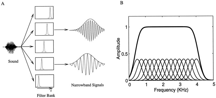
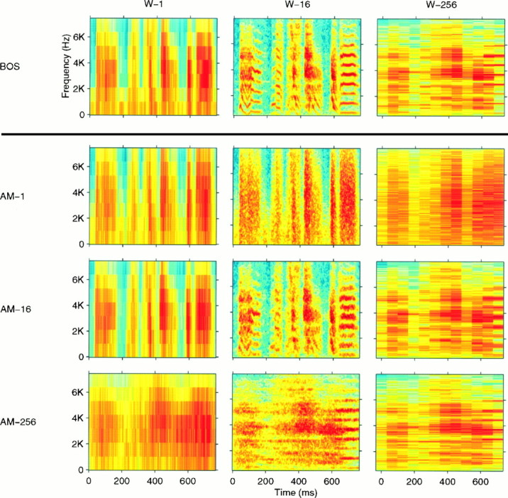
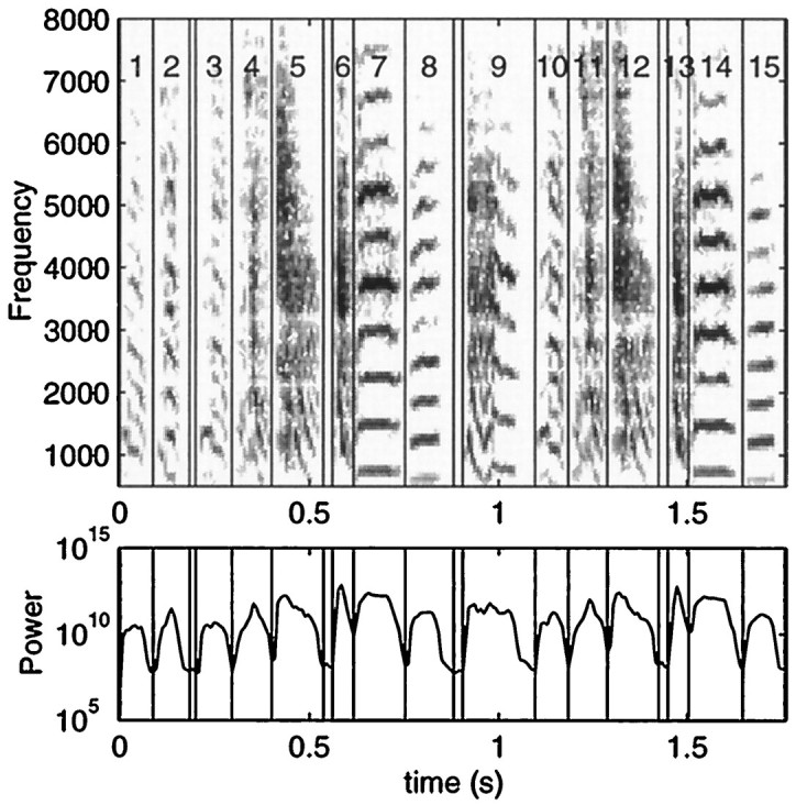
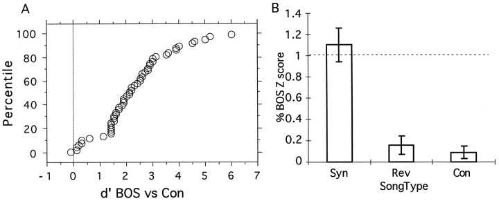
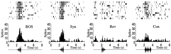
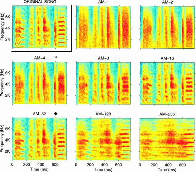
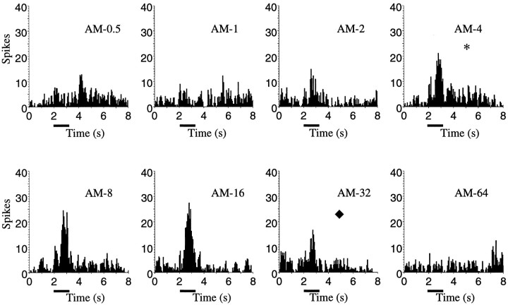
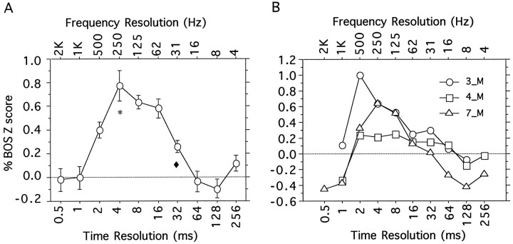
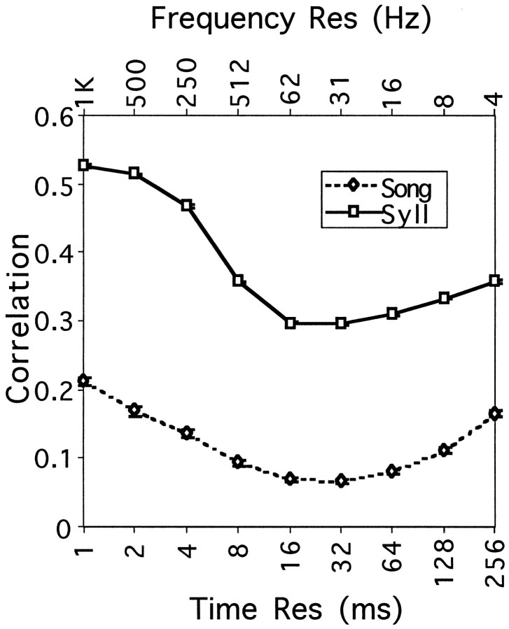
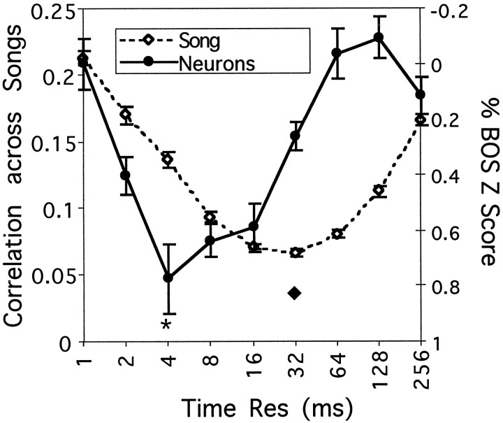
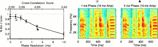
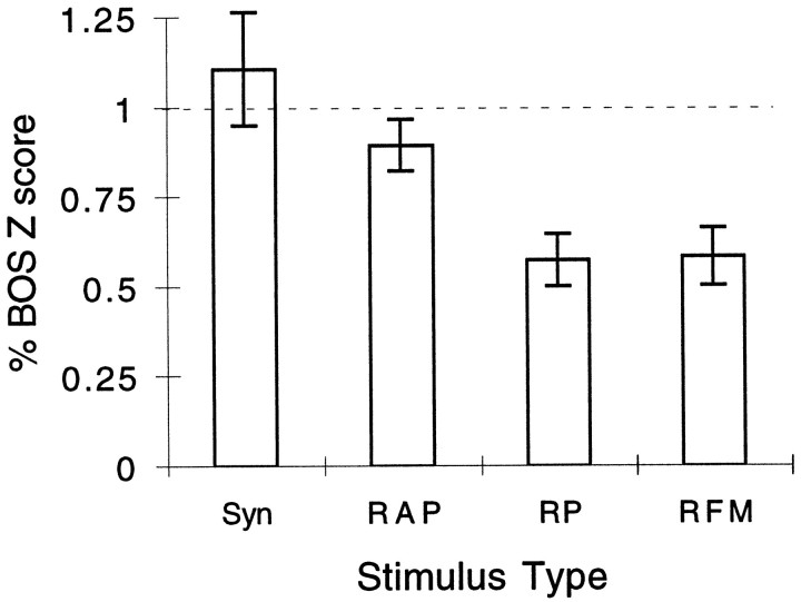
Complex vocalizations, such as human speech and birdsong, are characterized by their elaborate spectral and temporal structure. Because auditory neurons of the zebra finch forebrain nucleus HVc respond extremely selectively to a particular complex sound, the bird's own song (BOS), we analyzed the spectral and temporal requirements of these neurons by measuring their responses to systematically degraded versions of the BOS. These synthetic songs were based exclusively on the set of amplitude envelopes obtained from a decomposition of the original sound into frequency bands and preserved the acoustical structure present in the original song with varying degrees of spectral versus temporal resolution, which depended on the width of the frequency bands. Although both excessive temporal or spectral degradation eliminated responses, HVc neurons responded well to degraded synthetic songs with time-frequency resolutions of approximately 5 msec or 200 Hz. By comparing this neuronal time-frequency tuning with the time-frequency scales that best represented the acoustical structure in zebra finch song, we concluded that HVc neurons are more sensitive to temporal than to spectral cues. Furthermore, neuronal responses to synthetic songs were indistinguishable from those to the original BOS only when the amplitude envelopes of these songs were represented with 98% accuracy. That level of precision was equivalent to preserving the relative time-varying phase across frequency bands with resolutions finer than 2 msec. Spectral and temporal information are well known to be extracted by the peripheral auditory system, but this study demonstrates how precisely these cues must be preserved for the full response of high-level auditory neurons sensitive to learned vocalizations.

Fig. 1.

A, Schematic showing the decomposition of a complex sound into a set of narrowband signals, each described by an amplitude envelope and a frequency-modulated carrier. The complex sound is the input to a filter bank composed of a set of adjoining, and in this case overlapping, filters that cover the frequency range of interest. The narrowband output signals of two of the filters in the bank is shown. The envelope that was obtained with the analytical signal is drawn. The carrier frequency is centered at the frequency corresponding to the peak of the filter and has slow frequency modulations that are not easily discernible in this figure.B, Overall filter transform (thick line) obtained from a set of overlapping Gaussian filters (thin lines), the center frequencies of which are separated by one bandwidth (1 SD). The overall filter transform is almost perfectly flat for a large frequency range. In this example, we used 15 Gaussian filters with a bandwidth of 500 Hz and center frequencies between 500 and 4000 Hz.

Fig. 2.

Wideband (W-1), middleband (W-16), and narrowband (W-256) spectrograms generated with different time windows for a representative section of a zebra finch song motif (BOS) and three synthetic AM songs derived from that particular song (AM-1, AM-16, andAM-256). The time windows used to generate the spectrograms had a Gaussian shape and a width of 1, 16, or 256 msec, respectively. The three AM songs were generated by preserving the AM waveforms of the frequency decomposition of the original BOS obtained with a bank of Gaussian-shaped frequency filters, as explained in Materials and Methods. The filters also had widths of 1, 16, or 256 msec expressed in the time domain (1 kHz, 62.5 Hz, or 3.9 Hz, respectively, in the frequency domain). Therefore, theW-1 (W-16 andW-256) spectrogram for the AM-1(AM-16 and AM-256) song approximately matches the W-1 (W-16 andW-256, respectively) spectrogram for theBOS. At other time–frequency scales, the spectrograms of the AM songs do not match that of the BOS, illustrating the information that is lost in the AM songs. TheAM-1 song preserves the fine temporal modulations but does not have the frequency resolution of the BOS. TheAM-256 has good frequency discrimination calculated at longer time scales (notice the finer frequency bands for the last harmonic stack in the song) but has smeared the temporal structure present in the BOS. The AM-16 shows good time–frequency compromise.

Fig. 3.

Spectrogram (top) and overall power envelope (bottom) of one of the representative songs used in these experiments. The vertical lines are the divisions obtained from a computer program that automatically divides the song into syllable-like elements based on the peaks and troughs of the overall power (see Materials and Methods). Syllables 9–14 were chosen for the color spectrograms (see Figs. 2, 6).

Fig. 4.

A, Cumulative probability distribution of the measure d′ from signal detection theory for the discriminability between the BOS and conspecific songs (Con), calculated from the neural responses obtained at 54 recording sites. B, Response, measured as a percent of the response to the BOS, for the synthetic song that preserved all of the parameters obtained in our decomposition (Syn), for the song played in reverse (Rev), and for conspecific songs (Con). The data are obtained fromn = 30 for Syn,n = 39 for Rev, andn = 47 for Con (nrefers to the number of recording sites). The error bars show 1 SEM.

Fig. 5.

Individual spike rasters and peristimulus time histograms (top) for the response of a particular single unit in the HVc to the BOS, Syn,Rev, and Con stimuli (see Fig. 4). Oscillograms (waveform representations of the sound pressure) of the stimuli are shown below each histogram. Thed′ for this particular single unit was 1.5. As shown in Figure 4, ∼75% of the recording sites showed greater selectivity than did this particular neuron, and this neuron, despite its evident selectivity, is among the less selective members of the population that was used for the studies involving the synthetic stimuli (d′ > 1).

Fig. 6.

Spectrograms of a representative section of an original song and its corresponding degraded AM synthetic songs. The spectrograms of the AM-1 to AM-256 songs are shown. The songs generated with small time windows (1–4 msec) preserve the temporal modulations seen in the original song but have poor frequency resolution. For long time windows (such as 256 msec), the spectral resolution calculated at longer time scales is good, but the temporal structure present in the original signal is smeared. Thesymbols (*, ♦) indicate the time–frequency scale that gave the best neural response (*) and the best discrimination among songs (♦) (see Fig. 10 and the corresponding text). The samesymbols are also used below (see Figs. 7, 8). All spectrograms displayed in this figure were generated with 16 msec Gaussian windows.

Fig. 7.

Peristimulus histograms for a single-unit recording in response to the set of AM songs spanning the range of time–frequency scales between 0.5 and 64 msec. The responses to AM songs generated with time windows of >64 msec were similar to those obtained at 64 msec. The stimuli started at t = 2 sec and lasted ∼1 sec. This single unit and song were from bird zfa_18. This neuron is the same as that of Figure 5. Thesymbols (*, ♦) indicate the time–frequency scale that gave the best neural response (*) and the best discrimination among songs (♦) (see Figs. 6, 8, 10).

Fig. 8.

A, Time–frequency tuning curve of HVc in response to AM song stimuli. The x-axis shows the time (bottom) or frequency (top) scale that was used to generate the AM song stimuli. The response is measured as a percent of the response to the BOS. The error bars show 1 SEM. The number of recording sites for each stimulus was n = 31 for t = 0.5 msec, n = 31 fort = 1.0 msec, n = 42 fort = 2.0 msec, n = 35 fort = 4.0 msec, n = 41 fort = 8.0 msec, n = 37 fort = 16 msec, n = 42 fort = 32 msec, n = 33 fort = 64 msec, n = 40 fort = 128 msec, and n = 25 fort = 256 msec. The symbols (*, ♦) indicate the time–frequency scale that gave the best neural response (*) and the best discrimination among songs (♦) (see Figs. 6, 7, 10).B, Time–frequency tuning curves for three different single units from an individual bird. The x- andy-axes are identical to those in A.

Fig. 9.

Cross-correlation between amplitude envelopes calculated at different time–frequency scales for songs (Song) and syllables (Syll) from different birds. Sixteen different songs were used, resulting in 120 pairwise correlation measures for songs and over 2000 pairwise comparisons for syllables. Low values of cross-correlation indicate large differences between signals and therefore show the time–frequency scales that are best at discriminating among zebra finch songs. The error bars showing 1 SEM are smaller than the size of the markers.

Fig. 10.

Comparison of the cross-correlation measure for song similarity and of the response of HVc neurons as a function of the time–frequency scale. The data in Figures 8A and 9 are plotted together to facilitate the comparison. Note that theright y-axis for the neural response has been inverted and that the left y-axis for the cross-correlation among songs has been expanded. The symbols (*, ♦) indicate the time–frequency scale that gave the best neural response (*) and the best discrimination among songs (♦). The samesymbols are used in Figures 6-8.

Fig. 11.

Left, Mean HVc response curve to the synthetic songs that preserved the instantaneous relative phase across frequency bands with different degrees of accuracy. Thebottom x-axis shows the resolution expressed as 1 SD of relative phase noise (in units of milliseconds) that was added to each band. The top x-axis shows the normalized cross-correlation between the amplitude envelope of the synthetic songs and that of the original song. The error bars show 1 SEM. The number of recording sites for each point was n = 43 fort = 0.0 msec, n = 25 fort = 1.0 msec, n = 25 fort = 2.0 msec, n = 23 fort = 3.0 msec, n = 27 fort = 5.0 msec, and n = 26 fort = 10 msec. Middle,Right, Spectrograms of sections of a typical synthetic song with 1 msec (middle) and 5 msec (right) relative phase precision. The song shown is the same as that in Figures 2 and 6. The symbols are used to indicate the corresponding points in the leftcurve.

Fig. 12.

Mean HVc response curves to synthetic songs that had various amounts of FM noise added to each frequency band. Thex-axis shows the amount of noise expressed as 1 SD of the additive Gaussian noise. The RAP stimuli were generated by adding the same FM noise to each band and therefore preserving the relative instantaneous phase (n = 43 for FM = 0,n = 22 for FM = 1, n = 23 for FM = 5, n = 23 for FM = 15, andn = 25 for FM = 30). The RP stimuli had different FM noise added in each band (n = 28 for FM = 0, n = 24 for FM = 1,n = 25 for FM = 5, n = 15 for FM = 15, and n = 26 for FM = 30). For both cases, the absolute phase was random. The error bars show 1 SEM.

Fig. 13.

Summary response values for four synthetic songs that preserved various amounts of information embedded in the instantaneous phase. From right to left, the bars represent the average neural response to the following songs: RFM (random FM) is the AM song at 16 msec that has both random FM and absolute phase; RP song preserves the FM in each band but does not preserve the relative phase;RAP song has the correct FM and relative phase but random absolute phase; and Syn is the synthetic song in which all of the parameters are preserved. The error bars show 1 SEM. The number of recording sites for each stimulus wasn = 37 for RFM,n = 28 for RP, n= 43 for RAP, and n = 30 forSyn.

References

1. Brugge JF, Merzenich MM. Responses of neurons in auditory cortex of the macaque monkey to monaural and binaural stimulation. J Neurophysiol. 1973;36:1138–1158. - PubMed
1. Cohen L. Time-frequency analysis. Prentice Hall; Englewood Cliffs, NJ: 1995.
1. Dear SP, Fritz J, Haresign T, Ferragamo M, Simmons JA. Tonotopic and functional organization in the auditory cortex of the big brown bat, Eptesicus fuscus. J Neurophysiol. 1993;70:1988–2009. - PubMed
1. Delgutte B. Physiological models for basic auditory percepts. In: Hawkins HL, McMullen TA, Popper AN, Fay RR, editors. Auditory computation. Springer; New York: 1996. pp. 157–220.
1. Doupe AJ. Song and order selective neurons in the songbird anterior forebrain and their emergence during vocal development. J Neurosci. 1997;17:1147–1167. - PMC - PubMed
Publication types
LinkOut - more resources