Kinetic structure of large-conductance Ca2+-activated K+ channels suggests that the gating includes transitions through intermediate or secondary states. A mechanism for flickers

Abstract

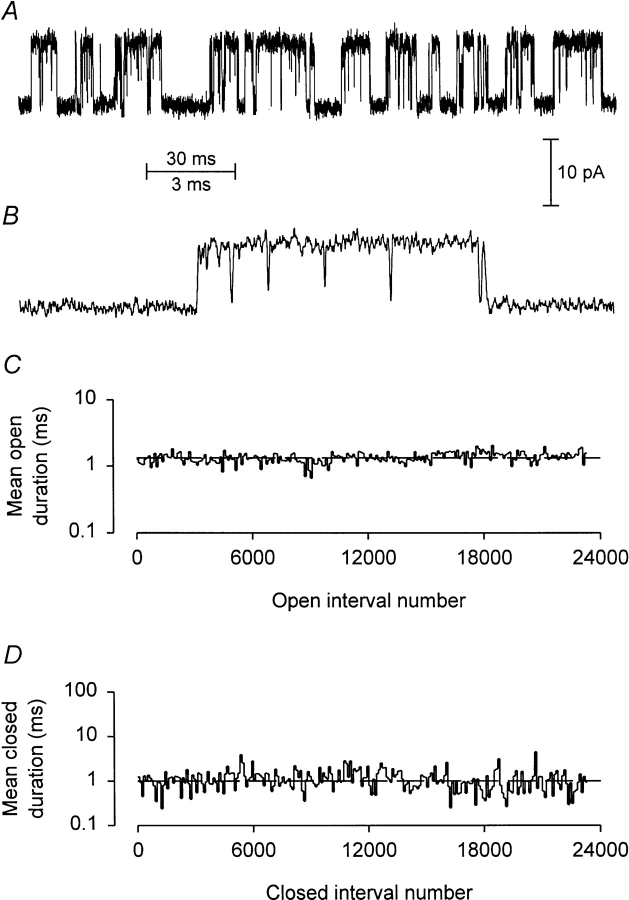
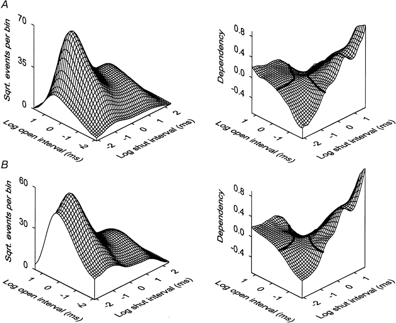
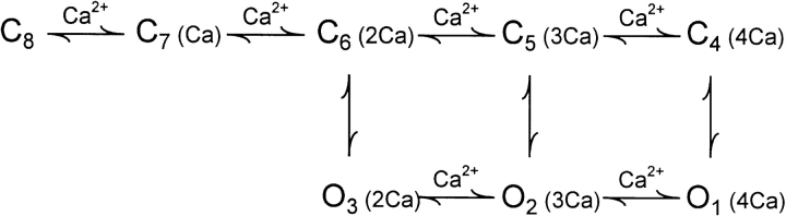
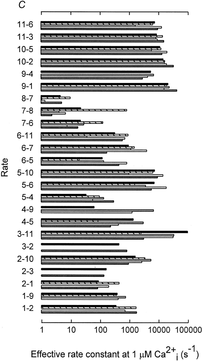
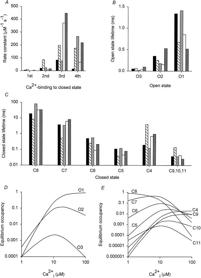
Mechanisms for the Ca2+-dependent gating of single large-conductance Ca2+-activated K+ channels from cultured rat skeletal muscle were developed using two-dimensional analysis of single-channel currents recorded with the patch clamp technique. To extract and display the essential kinetic information, the kinetic structure, from the single channel currents, adjacent open and closed intervals were binned as pairs and plotted as two-dimensional dwell-time distributions, and the excesses and deficits of the interval pairs over that expected for independent pairing were plotted as dependency plots. The basic features of the kinetic structure were generally the same among single large-conductance Ca2+-activated K+ channels, but channel-specific differences were readily apparent, suggesting heterogeneities in the gating. Simple gating schemes drawn from the Monod- Wyman-Changeux (MWC) model for allosteric proteins could approximate the basic features of the Ca2+ dependence of the kinetic structure. However, consistent differences between the observed and predicted dependency plots suggested that additional brief lifetime closed states not included in MWC-type models were involved in the gating. Adding these additional brief closed states to the MWC-type models, either beyond the activation pathway (secondary closed states) or within the activation pathway (intermediate closed states), improved the description of the Ca2+ dependence of the kinetic structure. Secondary closed states are consistent with the closing of secondary gates or channel block. Intermediate closed states are consistent with mechanisms in which the channel activates by passing through a series of intermediate conformations between the more stable open and closed states. It is the added secondary or intermediate closed states that give rise to the majority of the brief closings (flickers) in the gating.

Figure 1

Current records and stability plots from a single BK channel. (A and B) Current records at low and high time resolution recorded from an inside-out patch of membrane excised from cultured rat skeletal muscle. (C and D) Stability plots of the mean open and closed interval durations, averaged 100 at a time, after excluding any artifacts and shifts to modes other than normal. The effective low-pass filtering was 7.8 kHz; channel B12; membrane potential was +30 mV (intracellular membrane surface positive) in this and the following figures.

Figure 2

2-D dwell-time distributions for six different BK channels. Adjacent open and closed intervals were binned as pairs, with the logs of the open and closed interval durations locating the bins on the x and y axis, respectively. The z axis plots the square root of the number of interval pairs in each bin. The Ca²⁺ _i, open probabilities, numbers of plotted interval pairs in each distribution, and effective level of low-pass filtering were: channel B06: 12.3 μM, 0.50, 28,560, 6.3 kHz; B12: 12.3 μM, 0.54, 46,652, 7.8 kHz; B14: 12.3 μM, 0.61, 21,904, 10 kHz; M25: 21.6 μM, 0.52, 118,006, 5 kHz; M09: 7.46 μM, 0.58, 194,000, 6.3 kHz; M24: 23.1 μM, 0.52, 158,238, 7.3 kHz.

Figure 3

Dependency plots for six different BK channels. The fractional excess or deficit of interval pairs between the 2-D dwell-time distributions in Fig. 2 and the 2-D dwell-time distributions that would be expected for independent pairing of open and closed intervals is plotted as dependency (Eqs. 1 and 2). The heavy solid lines indicate a dependency of zero. Dependencies of +0.5 or −0.5 would indicate a 50% excess or deficit, respectively, of observed interval pairs over that expected for independent pairing of open and closed intervals.

Scheme I

Figure 4

Estimating the contribution of stochastic variation, filtering, and noise to the dependency plots. The 2-D dwell-time distribution for channel B06 in Fig. 2 was fitted with Scheme SI to obtain the most likely rate constants. These rate constants were then used with Scheme SI to simulate (with filtering and noise) the same number of detected interval pairs as for the plot for channel B06 in Fig. 2. The simulated single-channel current was then analyzed to obtain the predicted dwell-time distribution (A), the predicted dependency plot (B), and the predicted dependency significance (C). As expected for Scheme SI, which should have zero dependency, none of the dependencies were significant. The variation in dependency thus reflects contributions from stochastic variation, filtering, and noise.

Figure 5

Significance of the basic features of the dependency plots. (A) The significance of the dependencies in the dependency plots in Fig. 3 is plotted as dependency significance, which indicates the log of the P values times the sign of the dependency. Values of dependency significance greater than the heavy solid line at +1.3 and less than the heavy solid lines at −1.3 indicate that the dependency values are significant (P < 0.05). Absolute values of dependency significance >2, 3, and 4 would indicate P values < 0.01, < 0.001, and < 0.0001, respectively. (B) Backside views of the dependency significance plots in A for the indicated channels. There is a significant deficit of long closed intervals adjacent to long open intervals.

Figure 5

Significance of the basic features of the dependency plots. (A) The significance of the dependencies in the dependency plots in Fig. 3 is plotted as dependency significance, which indicates the log of the P values times the sign of the dependency. Values of dependency significance greater than the heavy solid line at +1.3 and less than the heavy solid lines at −1.3 indicate that the dependency values are significant (P < 0.05). Absolute values of dependency significance >2, 3, and 4 would indicate P values < 0.01, < 0.001, and < 0.0001, respectively. (B) Backside views of the dependency significance plots in A for the indicated channels. There is a significant deficit of long closed intervals adjacent to long open intervals.

Scheme II

Figure 6

Idealized 2-D dwell-time distributions and dependency plots for channel B06. The 2-D dwell-time distribution in Fig. 2 for channel B06 was fitted with the uncoupled Scheme SII. The estimated most likely rate constants were then used with Scheme SII to simulate a single-channel current with 10⁶ detected intervals that were then analyzed to obtain the 2-D dwell-time distribution and dependency plots. For A, the current was simulated with filtering and noise similar to that in the experimental record, and for B the current was simulated without filtering and noise. The effects of stochastic variation are removed by the large numbers of analyzed intervals. The differences between A and B indicate the effects of filtering and noise in A.

Figure 7

Ca²⁺ dependence of the kinetic structure. (A) Single-channel current records at the indicated Ca²⁺ _i. (B) 2-D dwell-time distributions and dependency plots. The numbers of pairs of intervals in the 2-D distributions for the indicated Ca²⁺ _i were: 5.5 μM, 10,168; 8.3 μM, 11,848; 12.3 μM, 28,560. (C) Idealized kinetic structures at the indicated Ca²⁺ _i, generated as described for Fig. 6 A. Channel B06.

Figure 7

Ca²⁺ dependence of the kinetic structure. (A) Single-channel current records at the indicated Ca²⁺ _i. (B) 2-D dwell-time distributions and dependency plots. The numbers of pairs of intervals in the 2-D distributions for the indicated Ca²⁺ _i were: 5.5 μM, 10,168; 8.3 μM, 11,848; 12.3 μM, 28,560. (C) Idealized kinetic structures at the indicated Ca²⁺ _i, generated as described for Fig. 6 A. Channel B06.

Figure 7

Ca²⁺ dependence of the kinetic structure. (A) Single-channel current records at the indicated Ca²⁺ _i. (B) 2-D dwell-time distributions and dependency plots. The numbers of pairs of intervals in the 2-D distributions for the indicated Ca²⁺ _i were: 5.5 μM, 10,168; 8.3 μM, 11,848; 12.3 μM, 28,560. (C) Idealized kinetic structures at the indicated Ca²⁺ _i, generated as described for Fig. 6 A. Channel B06.

Scheme III

Figure 8

Kinetic structure predicted by Scheme SIII for channel B06. The three 2-D dwell-time distributions in Fig. 7 B were simultaneously fitted with Scheme SIII to estimate the most likely rate constants. Scheme SIII with these rate constants and using noise and filtering similar to that in the experimental record was then used to generate the predicted kinetic structure at each Ca²⁺ _i. Scheme SIII captures the basic features of the kinetic structure, but has a number of deficiencies. Compare to Fig. 7, B and C. Channel B06.

Figure 9

Brief open and closed intervals can occur adjacent to each other. Typical examples of single-channel current records at 5.5 μM Ca²⁺ _i. *Adjacent brief open and closed intervals both within bursts and at the beginning and end of bursts. Channel B06.

Scheme IIIA

Figure 10

Kinetic structure predicted by Scheme IIIA for channel B06. The kinetic structures predicted by Scheme IIIA at the indicated Ca²⁺ _i are plotted for comparison to the observed kinetic structures in Fig. 7, B and C.

Figure 11

Single-channel currents predicted by Scheme IIIA for channel B06 for comparison to the experimental records in Figs. 7 A and 9. Idealized single-channel current records were generated, noise was added, and then the entire record was filtered with a four-pole digital Bessel filter to give the same effective dead time as that of the experimental record. (A) Simulated currents at the indicated Ca²⁺ _i. (B) Simulated currents on a faster time base showing selected examples of brief open intervals adjacent to brief closed intervals (5.5 μM Ca²⁺ _i). Simulated currents for Scheme IIIB for channel B06 appeared visually indistinguishable from the records in this figure after taking stochastic variation into account.

Figure 12

Estimated rate constants for Schemes III, IIIA, and IIIB. (A) Estimates of the rate constants for Scheme SIII are presented for five channels: B06 (black bar), B12 (hatched bar), B14 (light gray bar), M25 (white bar), and M09 (dark gray bar). (B) Estimates of the rate constants for Scheme IIIA for the same five channels. (C) Estimates of the rate constants for Scheme IIIB for the same five channels. Rate constants were estimated in each case by the simultaneous fitting of 2-D dwell-time distributions at three different Ca²⁺ _i.

Figure 12

Estimated rate constants for Schemes III, IIIA, and IIIB. (A) Estimates of the rate constants for Scheme SIII are presented for five channels: B06 (black bar), B12 (hatched bar), B14 (light gray bar), M25 (white bar), and M09 (dark gray bar). (B) Estimates of the rate constants for Scheme IIIA for the same five channels. (C) Estimates of the rate constants for Scheme IIIB for the same five channels. Rate constants were estimated in each case by the simultaneous fitting of 2-D dwell-time distributions at three different Ca²⁺ _i.

Scheme IIIB

Scheme IV

Scheme IVA

Scheme V

Scheme VA

Scheme VI

Scheme VIA

Scheme VII

Scheme VIIA

Figure 13

Kinetic structure predicted by Scheme VIA for channel M09. The kinetic structure predicted by Scheme VIA for channel M09 is presented for comparison to the observed structure in Figs. 2 and 3.

Figure 14

Gating of the BK channel according to Scheme IIIA. (A) Rate constants for the binding of the first through fourth Ca²⁺ for five channels, designated as in Fig. 12. Note the cooperativity in binding. (B) The lifetimes of the three open states increased progressively as the number of bound Ca²⁺ increased. (C) The lifetimes of closed states decreased as the number of bound Ca²⁺ increased, except for state C₄. States C₉, C₁₀, and C₁₁ were constrained to have the same lifetimes for any given channel. Hence, they are plotted as a group. (D and E) Predicted equilibrium occupancy as a function of Ca²⁺ _i for the indicated open and closed states in Scheme IIIA for channel B06.

References

1. Ackers GK, Doyle ML, Myers D, Daugherty MA. Molecular code for cooperativity in hemoglobin. Science. 1992;255:54–63. - PubMed
1. Adelman JP, Shen E, Kavanaugh MP, Warren RA, Wu Y, Lagrutta A, Bond C, North RA. Calcium-activated potassium channels expressed from cloned complementary DNAs. Neuron. 1992;9:209–216. - PubMed
1. Atkinson NS, Robertson GA, Ganetzky B. A component of calcium-activated potassium channels encoded by the Drosophila slo locus. Science. 1991;253:551–555. - PubMed
1. Auerbach A, Lingle CJ. Heterogeneous kinetic properties of acetylcholine receptor channels in Xenopus myocytes. J Physiol (Camb) 1986;378:119–140. - PMC - PubMed
1. Ball FG, Sansom MSP. Ion-channel gating mechanisms: model identification and parameter estimation from single channel recordings. Proc R Soc Lond B Biol Sci. 1989;236:385–416. - PubMed
Publication types